Spearman’s Rank Correlation Coefficient: While calculating the correlation coefficient or product-moment correlation coefficient, it is assumed that both characteristics are measurable. But, in reality, some characteristics are not measurable. For example,  the qualities of individuals are not measurable. Instead, they can be ranked based on their qualities. In such cases, rank correlation is used to determine the relationship between two characteristics.

Sometimes there will be no clear linear relationship between two random variables, but a monotonic relationship is evident. While Karl Pearson’s correlation coefficient indicates the strength of a linear relationship between two variables, Spearman’s rank correlation coefficient indicates the concentration of association between two qualitative characteristics.

LEARN EXAM CONCEPTS ON EMBIBE

Ranking and its Importance

In general, characteristics must be measurable to calculate the product-moment correlation coefficient. But some characteristics are not measurable in practical situations. This situation arises when dealing with qualitative studies such as honesty, beauty, and voice.

They are qualitative characteristics, and individuals or substances can be ranked according to their relative worth. A judge, for example, may rank contestants in a singing competition based on their performance. In another case, students may be ranked in different subjects based on their answers.

A ranking is the arrangement of individuals or items in order of merit or proficiency in possession of a specific characteristic, and rank is the number indicating the position of individuals or items.

What is Spearman’s Rank Correlation Coefficient?

If the ranks of individuals or items for two characteristics are available, the correlation between the ranks of these characteristics is known as rank correlation. We discover the relationship between two qualitative characteristics using rank correlation. Spearman’s rank correlation coefficient measures the strength of association between two ranked variables. 

Spearman’s Ranking of Data

The Spearman’s correlation coefficient, denoted by \(\rho \) or \({r_R}\), is a measure of the strength and the direction of the relationship between two ranked or ordered variables. This determines the degree to which a relationship is monotonic. In other words, whether the association between two ordered variables has a monotonic component.

Before starting with the Spearman’s Rank correlation evaluation, we must rank the data under consideration. This is necessary because we have to compare whether the other follows a monotonic relation on increasing one variable.

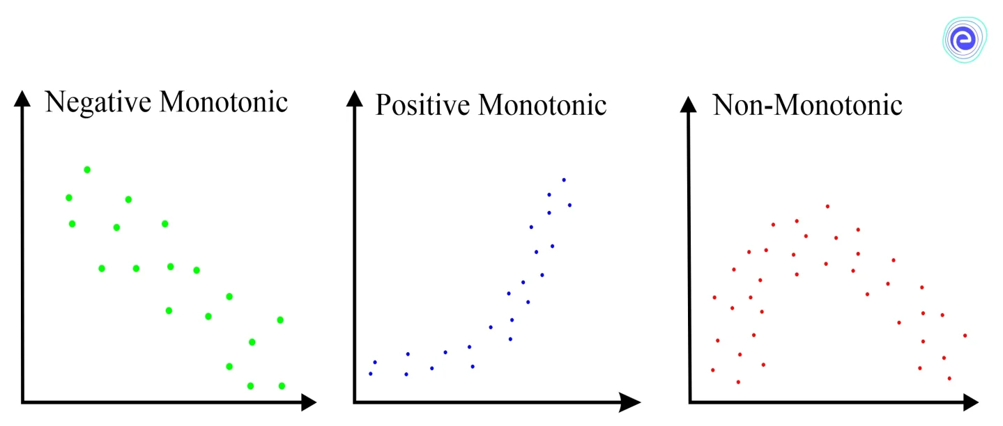
Each variable in a linear relationship changes in direction at the same rate throughout the data range. Each variable in a monotonic relationship changes in only one direction, but not necessarily at the same rate.

• Positive monotonic: when one variable rises, the other rises.

• Negative monotonic: when one variable rises, the other falls.

Thus, at every level, we have to compare the values of the two variables. This ranking method assigns levels to each value in the dataset, so we can easily compare them.

• Assign numbers \(1\) to \(n\), where \(n\) is the number of points corresponding to the values of variables in the order highest to smallest.
• If two or more data values are identical, assign the arithmetic mean of the ranks they would have occupied otherwise.

Example: 

Selling price values in ₹ of a product are \({\rm{28,32,19,22,20}}\) and \(22\). The highest value \(32\) is given the rank \(1\), while \(28\) is given rank \(2\), and so on. Two values are identical \((22)\). Hence, the arithmetic means of ranks that they would have otherwise occupied \(\frac{{3 + 4}}{2} = 3.5\) is taken. Hence, the corresponding ranks are: \(2,1,5,3.5,4,3.5\)

PRACTICE EXAM QUESTIONS AT EMBIBE

Interpretation of Spearman’s Rank Correlation Coefficient

The Spearman’s rank correlation coefficient, \(\rho \), ranges from \(+1\) to \(-1\)

• If the correlation coefficient is \(1\), then all of the rankings for each variable match up for every data pair.
• When the correlation coefficient is \(-1\), the rankings for one variable are the inverse of the rankings for the other variable.
• A correlation coefficient value close to \(0\) indicates that the variable rankings do not have a monotonic relationship.

Hence, in simpler words, we can say that,

• \(\rho = + 1\) denotes a perfect association of ranks
• \(\rho = 0\) denotes no association between ranks
• \(\rho = – 1\) denotes a perfect negative correlation of ranks.

The closer the value of \(\rho \) is to zero, the weaker the association or correlation between the ranks.

Formula of Spearman’s Rank Correlation Coefficient

The rank correlation coefficient is denoted by \(\rho \) or \({r_R}\) and is given by

\(\rho = {r_R} = 1 – \frac{{6\sum {d_i^2} }}{{n\left( {{n^2} – 1} \right)}}\)

Here,

\(\rho =\) the strength of the rank correlation between variables

\({d_i} = \) the difference between the \(x\) rank and the \(y\) rank for each pair of data

\(\sum {d_i^2} = \) sum of the squared differences between \(x\) and \(y\) variable ranks

\(n=\) sample size

Advantages and Disadvantages of Spearman’s Rank

Advantages	Disadvantages
Demonstrates the significance of the data	It can be difficult to find out
Correlation is proven or disproven	It is a fairly complicated formula
Allows for further investigation	It is possible to be misinterpreted
Do not make the assumption of normal distribution.	To run the test, you will need two sets of variable data

Solved Examples of Spearman’s Rank Correlation Coefficient

Q.1. Calculate the correlation coefficient between \(x\) & \(y\) for the following data given in the table below:

\(x\)	\(5\)	\(10\)	\(5\)	\(11\)	\(12\)	\(4\)	\(3\)	\(2\)	\(7\)	\(1\)
\(y\)	\(1\)	\(6\)	\(2\)	\(8\)	\(5\)	\(1\)	\(4\)	\(6\)	\(5\)	\(2\)

Ans:

Spearman’s correlation coefficient, \(r = \frac{{N\Sigma xy – (\Sigma x)(\Sigma y)}}{{\sqrt {N\Sigma {x^2} – {{(\Sigma x)}^2}} \times \sqrt {N\Sigma {y^2} – {{(\Sigma y)}^2}} }}\)

The table will be as follows.

\(x\)	\(y\)	\({x^2}\)	\({y^2}\)	\(xy\)
\(5\)	\(1\)	\(25\)	\(1\)	\(5\)
\(10\)	\(6\)	\(100\)	\(36\)	\(60\)
\(5\)	\(2\)	\(25\)	\(4\)	\(10\)
\(11\)	\(8\)	\(121\)	\(64\)	\(88\)
\(12\)	\(5\)	\(144\)	\(25\)	\(60\)
\(4\)	\(1\)	\(16\)	\(1\)	\(4\)
\(3\)	\(4\)	\(9\)	\(16\)	\(12\)
\(2\)	\(6\)	\(4\)	\(36\)	\(12\)
\(7\)	\(5\)	\(49\)	\(25\)	\(35\)
\(1\)	\(2\)	\(1\)	\(4\)	\(2\)
\(\Sigma x = 60\)	\(\Sigma x = 40\)	\(\Sigma {x^2} = 494\)	\(\Sigma {y^2} = 212\)	\(\Sigma xy = 288\)

Hence, the correlation coefficient

\(r = \frac{{10(288) – (60)(40)}}{{\sqrt {10(494) – {{(60)}^2}} \sqrt {10(212) – {{(40)}^2}} }}\)

\( = \frac{{2880 – 2400}}{{\sqrt {1340} \cdot \sqrt {520} }}\)

\( = \frac{{480}}{{(36.61)(22.80)}}\)

\( = \frac{{480}}{{834.71}}\)

\(\therefore r = 0.575\)

Hence, we can see that the variables \(x\) and \(y\) are positively correlated.

Q.2. Three judges in a beauty contest assess five persons. We have to find out which pair of judges have the nearest approach to the common perception of beauty.

Judge	Competitor \(1\)	Competitor \(2\)	Competitor \(3\)	Competitor \(4\)	Competitor \(5\)
\(A\)	\(1\)	\(2\)	\(3\)	\(4\)	\(5\)
\(B\)	\(2\)	\(4\)	\(1\)	\(5\)	\(3\)
\(C\)	\(1\)	\(3\)	\(5\)	\(2\)	\(4\)

Ans:

Correlation coefficient formula, \({r_S} = 1 – \frac{{6\Sigma {D^2}}}{{{n^3} – n}}\)

The rank correlation between \(A\) and \(B\) is calculated as follows:

\(A\)	\(B\)	\(D\)	\({D^2}\)
\(1\)	\(2\)	\(-1\)	\(1\)
\(2\)	\(4\)	\(-2\)	\(4\)
\(3\)	\(1\)	\(2\)	\(4\)
\(4\)	\(5\)	\(-1\)	\(1\)
\(5\)	\(3\)	\(2\)	\(4\)
		Total	\(14\)

\( \Rightarrow {r_s} = 1 – \frac{{6 \times 14}}{{{5^3} – 5}}\)

\( = 1 – \frac{{84}}{{120}}\)

\( = 1 – 0.7\)

\(\therefore {r_s} = 0.3\)

The rank correlation between \(A\) and \(C\) is calculated as follows:

\(A\)	\(C\)	\(D\)	\({D^2}\)
\(1\)	\(1\)	\(0\)	\(0\)
\(2\)	\(3\)	\(-1\)	\(1\)
\(3\)	\(5\)	\(-2\)	\(4\)
\(4\)	\(2\)	\(2\)	\(4\)
\(5\)	\(4\)	\(1\)	\(1\)
Total			\(10\)

\( \Rightarrow {r_s} = 1 – \frac{{6 \times 10}}{{{5^3} – 5}}\)

\( = 1 – \frac{{60}}{{120}}\)

\( = 1 – 0.5\)

\(\therefore {r_s} = 0.5\)

Similarly, the rank correlation between the rankings of judges\(B\) and \(C\) is

\(B\)	\(C\)	\(D\)	\({D^2}\)
\(2\)	\(1\)	\(1\)	\(1\)
\(4\)	\(3\)	\(1\)	\(1\)
\(1\)	\(5\)	\(-4\)	\(16\)
\(5\)	\(2\)	\(3\)	\(9\)
\(3\)	\(4\)	\(-1\)	\(1\)
		Total	\(28\)

\({{\rm{r}}_{\rm{s}}} = 1 – \frac{{6 \times 28}}{{{5^3} – 5}}\)

\( = 1 – \frac{{168}}{{120}}\)

\( = 1 – 1.4\)

\(\therefore {r_s} = – 0.4\)

Thus, the perceptions of judges \(A\) and \(C\) are the closest. Judges \(B\) and \(C\) have very different tastes.

Q.3. The table below provides data about the percentage of students who get meals at university and their CGPA marks. Calculate the Spearman’s Rank Correlation between the percentage of the students and their CGPA and interpret the result.

State University	\(\%\) of students having meals	\(\%\) of students scoring above \(8.5\) CGPA
Pune	\(14.4\)	\(54\)
Chennai	\(7.2\)	\(64\)
Delhi	\(27.5\)	\(44\)
Kanpur	\(33.8\)	\(32\)
Ahmedabad	\(38.0\)	\(37\)
Indore	\(15.9\)	\(68\)
Guwahati	\(4.9\)	\(62\)

Ans:

Let, \(X\) represent the \(\%\) of students having meals and

\(y\) represent the \(\%\) of students scored CGPA above \(8.5\).

State University	\({d_x} = {\text{Rank}}{{\text{s}}_x}\)	\({d_y} = {\text{Rank}}{{\text{s}}_{\text{y}}}\)	\(d = \left( {{d_x} – {d_y}} \right)\)	\({d^2}\)
Pune	\(3\)	\(4\)	\(-1\)	\(1\)
Chennai	\(2\)	\(6\)	\(-4\)	\(16\)
Delhi	\(5\)	\(3\)	\(2\)	\(4\)
Kanpur	\(6\)	\(1\)	\(5\)	\(25\)
Ahmedabad	\(7\)	\(2\)	\(5\)	\(25\)
Indore	\(4\)	\(7\)	\(-3\)	\(9\)
Guwahati	\(1\)	\(5\)	\(-4\)	\(16\)
				\(\Sigma {{\rm{d}}^2} = 96\)

\({r_s} = 1 – \frac{{6{\Sigma _i}d_i^2}}{{n\left( {{n^2} – 1} \right)}}\)

Now, using the formula with \(n=7\),

\( \Rightarrow {r_s} = 1 – \frac{{6.96}}{{7 \cdot (49 – 1)}}\)

\( = 1 – \frac{{576}}{{336}}\)

\(\therefore {r_s} = – 0.714\)

The value of \(r\) indicates a strong negative coefficient of correlation. It means that the universities with the highest percentage of students consuming meals tend to have the least successful results (and vice-versa).

Q.4. Suppose we have ranks of \(8\) students with B.Sc. in Statistics & Mathematics. On the basis of ranks, find to what extent the student’s knowledge in Statistics and Mathematics is related.

Rank in Statistics	\(1\)	\(2\)	\(3\)	\(4\)	\(5\)	\(6\)	\(7\)	\(8\)
Rank in Mathematics	\(2\)	\(4\)	\(1\)	\(5\)	\(3\)	\(8\)	\(7\)	\(6\)

Ans:

Spearman’s rank correlation coefficient formula is

\({r_s} = 1 – \frac{{6\sum\limits_{i = 1}^n {d_i^2} }}{{n\left( {{n^2} – 1} \right)}}\)

Rank in Statistics \(\left( {{R_x}} \right)\)	Rank in Mathematics \(\left( {{R_y}} \right)\)	Difference of Ranks \(\left( {{d_i} = {R_x} – {R_y}} \right)\)	\(d_i^2\)
\(1\)	\(2\)	\(-1\)	\(1\)
\(2\)	\(4\)	\(-2\)	\(4\)
\(3\)	\(1\)	\(2\)	\(4\)
\(4\)	\(5\)	\(-1\)	\(1\)
\(5\)	\(3\)	\(2\)	\(4\)
\(6\)	\(8\)	\(-2\)	\(4\)
\(7\)	\(7\)	\(0\)	\(0\)
\(8\)	\(5\)	\(2\)	\(4\)
			\(\sum {d_i^2} = 22\)

Here, number of paired observations, \(n=8\)

\({r_{\rm{s}}} = 1 – \frac{{6\sum {{\rm{d}}_{\rm{i}}^2} }}{{{\rm{n}}\left( {{{\rm{n}}^2} – 1} \right)}}\)

\( = 1 – \frac{{6 \times 22}}{{8 \times 63}}\)

\( = 1 – \frac{{132}}{{504}}\)

\( = \frac{{372}}{{504}}\)

\(\therefore {r_s} = 0.74\)

Thus the value of \({\gamma _{\rm{S}}}\) shows that there is a positive association between the ranks of Statistics and Mathematics.

Q.5. Calculate the rank correlation coefficient between \(X\) and \(Y\) from the following data.

\(X\)	\(78\)	\(89\)	\(97\)	\(69\)	\(59\)	\(79\)	\(68\)
\(Y\)	\(125\)	\(137\)	\(156\)	\(112\)	\(107\)	\(136\)	\(124\)

Ans:

To find the correlation coefficient, we need to do some calculations and extend the given table as below.

\(x\)	\(y\)	Rank of \(x\left( {{R_x}} \right)\)	Rank of \(y\left( {{R_y}} \right)\)	\(d = {R_x} – {R_y}\)	\({d^2}\)
\(78\)	\(125\)	\(4\)	\(4\)	\(0\)	\(0\)
\(89\)	\(137\)	\(2\)	\(2\)	\(0\)	\(0\)
\(97\)	\(156\)	\(1\)	\(1\)	\(0\)	\(0\)
\(69\)	\(112\)	\(5\)	\(6\)	\(-1\)	\(1\)
\(59\)	\(107\)	\(7\)	\(7\)	\(0\)	\(0\)
\(79\)	\(136\)	\(3\)	\(3\)	\(0\)	\(0\)
\(68\)	\(124\)	\(6\)	\(5\)	\(1\)	\(1\)
					\(\sum\limits_{i = 1}^n {d_i^2} = 2\)

Spearman’s Rank correlation formula is

\({r_s} = 1 – \frac{{6\sum\limits_{i = 1}^n {d_i^2} }}{{n\left( {{n^2} – 1} \right)}}\)

\({r_s} = 1 – \frac{{6 \times 2}}{{7(49 – 1)}}\)

\( = 1 – \frac{{12}}{{7 \times 48}}\)

\( = 1 – \frac{1}{{28}}\)

\( = \frac{{27}}{{28}}\)

\(\therefore {r_s} = 0.96\)

Summary

The common alternative to Karl Pearson’s \(r\) is Spearman’s \(\rho \). It is also known as Spearman’s rank correlation coefficient. It is a rank correlation coefficient as it uses the rankings of data of each variable rather than the raw data. When the data do not qualify the assumptions or requirements of Pearson’s \(r\) Spearman’s \(\rho \) is used.

This occurs when at least one of your variables is measured on an ordinal scale or when one or more variable’s data does not follow normal distributions. The Pearson correlation coefficient measures relationship linearity, while the Spearman correlation coefficient measures relationship monotonicity.

FAQs on Spearman’s Rank Correlation Coefficient

Students must have many questions with respect to Spearman’s Rank Correlation Coefficient. Here are a few commonly asked questions and answers.

Q.1. What is Spearman’s rank correlation coefficient used for?
Ans: Spearman’s rank correlation coefficient measures the strength and direction of association between two ranked variables. It is simple to understand and calculate. If we want to see the relationship between qualitative characteristics, the only formula we have is the rank correlation coefficient.

Q.2. How to calculate Spearman’s rank correlation coefficient?
Ans: The rank correlation coefficient is denoted by \(\rho \) or \({r_S}\) and can be calculated using the formula
\(\rho = {r_S} = 1 – \frac{{6\sum {d_i^2} }}{{n\left( {{n^2} – 1} \right)}}\)
Here,
\(\rho =\) the strength of the rank correlation between variables
\({d_i} = \) the difference between the \(x\) rank and the \(y\) rank for each pair of data
\(\sum {d_i^2} = \) sum of the squared differences between \(x\) and \(y\) variable ranks
\(n=\) sample size

Q.3. What is Spearman’s rank-order coefficient of correlation?
Ans: Spearman’s rank correlation coefficient is a non-parametric measure of rank correlation. It evaluates how well the association between two variables can be depicted using a monotonic function.

Q.4. How do you do Spearman rank with tied ranks?
Ans: When we have tied ranks or repeated ranks, we take the mean or average of the same ranks.

Q.5. What is the difference between Spearman’s and Karl Pearson’s coefficient of correlation?
Ans: Karl Pearson’s correlation coefficient indicates the strength of a linear relationship between two variables, whereas Spearman’s rank correlation coefficient indicates the concentration of association between two qualitative characteristics. On the other hand, Spearman’s rank correlation coefficient measures the strength of association between two ranked variables. 

LEARN EXAM CONCEPTS ON EMBIBE

We hope this information about Spearman’s Rank Correlation Coefficient has been helpful. If you have any doubts, comment in the section below, and we will get back to you soon.