Correlation Coefficient: Correlation investigates the relationship, or association, between two variables by examining how the variables change about one another. Correlation analysis is a method for systematically examining relationships between two variables.

It addresses issues such as whether there is a relationship between two variables, the change in the value of a variable or the other, whether both variables move in the same direction and how strong the relationship is. Correlation investigates and quantifies the direction and strength of relationships between variables. Scatter diagrams and the coefficient of correlation are two important tools for studying correlation.

Correlation Coefficient: What is it?

Statistical Correlation also refers to changes in two variables that occur simultaneously, and linear relationships represent it. Importantly, correlation does not always imply causation. This is because a correlation describes how two or more variables are related rather than whether they cause changes in each other.
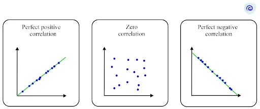
Correlation coefficient expresses the degree of association between two quantitative variables. It evaluates the strength of the relationship between the relative movements of the two variables. The values range from \(-1\) to \(+1\). A coefficient value greater than \(1\) or less than \(-1\) indicates incorrect measurement. A correlation of \(-1\) indicates a perfect negative correlation, while a correlation of \(1.0\) indicates a perfect positive correlation. A correlation of \(0\) indicates the absence of a linear relationship between the two variables.

Correlation Coefficient Value	Correlation Type	Meaning
\(+1\)	Perfect Positive correlation	When one variable changes, the other changes in the same direction.
\(0\)	Zero Correlation	There is no connection between the variables.
\(-1\)	Perfect Negative Correlation	When one variable changes, the other changes in the opposite direction.

Interpretation of Correlation Coefficient

The correlation coefficient, typically denoted by \(r\), is a real number between \(-1\) and \(1\). The value of r measures the strength of a correlation based on a formula, eliminating any subjectivity in the process. 

The sign of the correlation coefficient indicates whether the variables change in the same or opposite directions.

• A positive value indicates that the variables change in the same direction
• A negative value indicates that they change in opposite directions

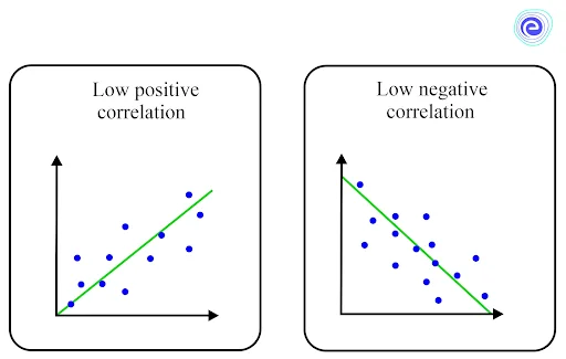
A correlation coefficient’s absolute value indicates the magnitude of the correlation. The greater the absolute value, the stronger will be their correlation. There are different sets of guidelines for interpreting the correlation coefficient because findings vary between study fields.

Some key points to understand when interpreting the value of \(r\) are listed below:

• If \(r=0,\) the points are a complete jumble with no linear relationship.
• If \(r=-1\) or \(r=1,\) then all data points line up perfectly on a line.
• If \(r\) is a value other than the extremes, the result is less than a perfectly straight line.
• If \(r\) is positive, then the line is going up with a positive slope. If \(r\) is negative, then the line is going down with a negative slope.

Correlation Coefficient	Correlation Strength	Correlation Type
\(-0.7\) to \(-1\)	Very strong	Negative
\(-0.5\) to \(-0.7\)	Strong	Negative
\(-0.3\) to \(-0.5\)	Moderate	Negative
\(0\) to \(-0.3\)	Weak	Negative
\(0\)	None	Zero
\(0\) to \(0.3\)	Weak	Positive
\(0.3\) to \(0.5\)	Moderate	Positive
\(0.5\) to \(0.7\)	Strong	Positive
\(0.7\) to \(1\)	Very strong	Positive

The correlation coefficient depicts how well the data fits on a line. If there is a linear relationship on a scatter plot, a straight line of best fit that considers all the data points can be drawn.

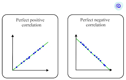
The greater the absolute value of the correlation coefficient, the stronger the linear correlation, and the closer your points are to the line. A perfect correlation exists when all points are perfectly on the line.

If all your points are close to the line, your correlation coefficient has a high absolute value.

The absolute value or value without sign of the coefficient of correlation is low if a large distance separates these points from this line.

Note that the steepness or slope of the line has nothing to do with the correlation coefficient value.

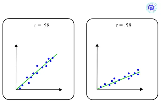
As two datasets with the same value of correlation coefficient can have lines with very different slopes, the correlation coefficient does not help predict how much one variable will vary based on a given change in the other.

Formulas of Coefficient of Correlation

The most commonly used methods of calculating the coefficient of correlation are:

• Karl Pearson’s Coefficient of Correlation
• Spearman’s Rank Correlation Coefficient

Karl Pearson’s Coefficient of Correlation

Karl Pearson’s correlation coefficient is a common mathematical method wherein the numerical expression calculates the degree and direction of the relationship between related linear variables. The linear relationship between two variables is measured by this correlation. However, it cannot differentiate between independent and dependent variables. The stronger the correlation between two datasets, the closer will be the coefficient value to \(+1\) or \(-1.\)

The Karl Pearson’s measure of correlation, is given by

\(r = \frac{\sum xy}{{N{\sigma _x}{\sigma _y}}}\)

Or 

\(r = \frac{{\sum {\left( {X – \overline X } \right)\left( {Y -\overline Y } \right)} }}{{\sqrt {\sum {{{\left( {X – \overline X } \right)}^2}} } \sqrt {\sum {{{\left( {Y – \overline Y } \right)}^2}} } }}\)

Where 

\(\overline X \) and \(\overline Y\) are the arithmetic means of \(X\) and \(Y\)

\(\sigma\) is the standard deviation

Spearman’s Rank Correlation Coefficient

Spearman’s rank correlation coefficient is used in cases where the relationship is non-linear. It is used to determine the monotony of two sets of data. This measurement is based on the ranked values for each dataset and employs skewed variables. Extreme values do not affect Spearman’s correlation coefficient.

As a result, if the data contains some outliers, Spearman’s correlation coefficient can be incredibly useful. The formula to find the Spearman’s rank coefficient is 

\({r_a} = 1 – \frac{{6\mathop \sum {D^2}}}{{{n^3} – n}}\)

Here, \(n\) is the number of observations, and \(D\) is the deviation of ranks assigned to a variable from those assigned to the other variable.

Solved Examples – Correlation Coefficient

Here are few solved examples of Correlation Coefficient for in depth idea

Q1. Calculate the coefficient of correlation of the age of husbands and wives in a village in Karnataka using Karl Pearson’s method.

Age of Husbands	\(23\)	\(27\)	\(28\)	\(29\)	\(30\)	\(31\)	\(33\)	\(35\)	\(36\)
Age of Wives	\(18\)	\(20\)	\(22\)	\(27\)	\(29\)	\(27\)	\(29\)	\(28\)	\(29\)

Solution:

Let the age of the husbands be denoted by \(h\) and the age of the wives be denoted by \(w.\) The necessary values can be obtained from the table.

Mean age of husbands \(\overline H = \frac{{\sum h}}{n} = \frac{{272}}{9} = 30.22\)

Mean age of wives \(\overline W = \frac{{\sum w}}{n} = \frac{{229}}{9} = 25.44\)

\(h\)	\(h = H – \overline H \)	\({h^2}\)	\(w\)	\(w = W – \overline W\)	\({w^2}\)	\(hw\)
\(23\)	\(-7.22\)	\(52.12\)	\(18\)	\(-7.44\)	\(55.35\)	\(53.71\)
\(27\)	\(-3.22\)	\(10.36\)	\(20\)	\(-5.44\)	\(29.59\)	\(17.51\)
\(28\)	\(-2.22\)	\(4.92\)	\(22\)	\(-3.44\)	\(11.83\)	\(7.63\)
\(29\)	\(-1.22\)	\(1.48\)	\(27\)	\(1.56\)	\(2.43\)	\(-1.90\)
\(30\)	\(-0.22\)	\(0.04\)	\(29\)	\(3.56\)	\(12.67\)	\(-0.78\)
\(31\)	\(0.78\)	\(0.60\)	\(27\)	\(1.56\)	\(2.43\)	\(1.21\)
\(33\)	\(2.78\)	\(7.72\)	\(29\)	\(3.56\)	\(12.67\)	\(9.89\)
\(35\)	\(4.78\)	\(22.84\)	\(28\)	\(2.56\)	\(6.55\)	\(12.23\)
\(36\)	\(5.78\)	\(33.40\)	\(29\)	\(3.56\)	\(12.67\)	\(20.57\)
\(\sum h = 272\)		\(\sum {h^2} = 133.48\)	\(\sum w = 229\)		\(\sum {w^2} = 146.19\)	\(\sum wh = 120.07\)

Hence, the correlation coefficient \(r = \frac{{\sum wh}}{{\sqrt {\sum {h^2} \times \sum } {w^2}}}\) 

\(r = \frac{{120.17}}{{\sqrt {133.48 \times 146.19} }}\)

\(∴r=0.86\)

Q2. Find the correlation coefficient between a man’s age and his glucose levels.

Sl.No.	Age \((x)\)	Glucose Level \((y)\)
\(1\)	\(42\)	\(98\)
\(2\)	\(23\)	\(68\)
\(3\)	\(22\)	\(73\)
\(4\)	\(47\)	\(79\)
\(5\)	\(50\)	\(88\)
\(6\)	\(60\)	\(82\)

Solution:

No.	Age \((x)\)	Glucose Level \((y)\)	\(xy\)	\({x^2}\)	\({y^2}\)
\(1\)	\(42\)	\(98\)	\(4116\)	\(1764\)	\(9604\)
\(2\)	\(23\)	\(68\)	\(1564\)	\(529\)	\(4624\)
\(3\)	\(22\)	\(73\)	\(1606\)	\(484\)	\(5329\)
\(4\)	\(47\)	\(79\)	\(3713\)	\(2209\)	\(6241\)
\(5\)	\(50\)	\(88\)	\(4400\)	\(2500\)	\(7744\)
\(6\)	\(60\)	\(82\)	\(4980\)	\(3600\)	\(6724\)
	\(\sum x = 244\)	\(\sum y = 488\)	\(\sum x y = 20379\)	\(\sum {{x^2}} = 11086\)	\(\sum {{y^2}} = 40266\)

\(r = \frac{{n\left( {\sum x y} \right) – \left( {\sum x } \right)\left( {\sum y } \right)}}{{\sqrt {\left[ {n\sum {{x^2}} – {{\left( {\sum x } \right)}^2}} \right]\left[ {n\sum {{y^2}} – {{\left( {\sum y } \right)}^2}} \right]} }}\) 

\(r = \frac{{6 \times 20379 – (244)(488)}}{{\sqrt {\left[ {6(11086) – {{(244)}^2}} \right]\left[ {6(40266) – {{(488)}^2}} \right]} }}\)  

\(r = \frac{{3202}}{{\sqrt {6980 \times 3452} }}\) 

\(r = \frac{{3202}}{{4972.238}}\)

\(∴r=0.6439\)

Q3. Calculate the correlation coefficient indicating the association between age and weight from the data given in the following table:

Subject	Age \(x\)	Weight \(y\)
\(1\)	\(40\)	\(99\)
\(2\)	\(25\)	\(79\)
\(3\)	\(22\)	\(69\)
\(4\)	\(54\)	\(89\)

Solution:

Subject	Age \(x\)	Weight \(y\)	\(xy\)	\({x^2}\)	\({y^2}\)
\(1\)	\(40\)	\(99\)	\(3960\)	\(1600\)	\(9801\)
\(2\)	\(25\)	\(79\)	\(1975\)	\(625\)	\(6241\)
\(3\)	\(22\)	\(69\)	\(1518\)	\(484\)	\(4761\)
\(4\)	\(54\)	\(89\)	\(4806\)	\(2916\)	\(7921\)
∑	\(151\)	\(336\)	\(12259\)	\(5625\)	\(28724\)

\(r = \frac{{n\left( {\sum x y} \right) – \left( {\sum x } \right)\left( {\sum y } \right)}}{{\sqrt {\left[ {n\sum {{x^2}} – {{\left( {\sum x } \right)}^2}} \right]\left[ {n\sum {{y^2}} – {{\left( {\sum y } \right)}^2}} \right]} }}\)

\( \Rightarrow r = \frac{{4(12258) – (151)(336)}}{{\sqrt {\left[ {4(5625) – {{(151)}^2}} \right]\left[ {4(28724) – {{(336)}^2}} \right]} }}\)

\( \Rightarrow r = \frac{{ – 1704}}{{\sqrt {[ – 301][ – 2000]} }}\)

\( \Rightarrow r = \frac{{ – 1704}}{{775.886}}\)

\(∴r=-2.1961\)

Q4. Calculate the correlation coefficient between \(X\) and \(Y\) from the following data given in the table.

\(X\)	\(Y\)
\(7\)	\(17\)
\(9\)	\(19\)
\(14\)	\(21\)

Solution:

\(X\)	\(Y\)	\(XY\)	\({X^2}\)	\({Y^2}\)
\(7\)	\(17\)	\(119\)	\(49\)	\(36\)
\(9\)	\(19\)	\(171\)	\(81\)	\(361\)
\(14\)	\(21\)	\(294\)	\(196\)	\(141\)
\(\sum X = 30\)	\(\sum Y = 57\)	\(\sum X Y = 584\)	\({\sum X ^2} = 326\)	\(\sum {{Y^2}} = 838\)

\(r = \frac{{n\left( \sum {xy} \right) – \left( \sum x \right)\left( {\sum y} \right)}}{{\sqrt {\left[ {n\sum {x^2} – {{\left( {\sum x} \right)}^2}} \right]\left[ {n\sum {y^2} – {{\left( {\sum y} \right)}^2}} \right]} }}\) 

\( \Rightarrow r = \frac{{3(584) – (30)(57)}}{{\sqrt {\left[ {3(326) – {{(30)}^2}} \right]\left[ {3(838) – {{(57)}^2}} \right]} }}\)

\( \Rightarrow r = \frac{{42}}{{\sqrt {[78][ – 735]} }}\)

\( \Rightarrow r = \frac{{42}}{{ – 239.43}}\)

\(∴r=-0.1754\)

Q5. The sample data of a person’s age and their corresponding income is shown in the table given below. Find out whether the increase in age influences income using the correlation coefficient formula.

Age	\(25\)	\(30\)	\(46\)	\(43\)
Income	\(30000\)	\(44000\)	\(52000\)	\(7000\)

Solution:

Let age is denoted by \(x\) and income be denoted by \(y.\) To simplify the calculation, let us divide \(y\) by \(1000.\)

Age \(\left( {{x_i}} \right)\)	\(\frac{{{\text{income}}}}{{1000}}\)\(\left( {\frac{{{y_i}}}{{1000}}} \right)\)	\({x_i} – \overline x \)	\({y_i} – \overline y \)	\({\left( {{x_i} – \overline x } \right)^2}\)	\({\left( {{y_i} – \overline y } \right)^2}\)	\(\left( {{x_i} – \overline x } \right)\left( {{y_i} – \overline y } \right)\)
\(25\)	\(30\)	\(-8.5\)	\(-19\)	\(72.25\)	\(361\)	\(161.5\)\(
\(30\)	\(44\)	\(-3.5\)	\(-5\)	\(12.25\)	\(25\)	\(17.5\)
\(36\)	\(52\)	\(2.5\)	\(3\)	\(6.25\)	\(9\)	\(7.5\)
\(43\)	\(70\)	\(70\)	\(21\)	\(90.25\)	\(441\)	\(199.5\)
\(\underline x = 33.5\)	\(\underline y = 49\)			\(\sum {\left( {{x_i} – \underline x } \right)^2} = 181\)	\(\sum {\left( {{y_i} – \underline y} \right)^2} = 836\)	\(\sum \left( {{x_i} – \underline x } \right)\left( {{y_i} – \underline y } \right) = 386\)

\(r = \frac{{\sum {\left( {{x_i} – \overline x } \right)} \left( {{y_i} – \overline y } \right)}}{{\sqrt {\sum {{{\left( {{x_i} – \overline x } \right)}^2}} \sum {{{\left( {{y_i} – \overline y } \right)}^2}} } }}\)

\( = \frac{{386}}{{\sqrt {181} \sqrt {836} }}\)

\( = \frac{{193}}{{\sqrt {181} \sqrt {209} }}\)

\(∴r=0.99\)

The value of the correlation coefficient \(r\) is close to \(1.\) Hence we can say that the person’s income increases with age.

Summary

Correlation is a statistical measure that expresses how closely two variables are related linearly. It is a standard tool for describing relationships without stating a cause and effect. The correlation coefficient is a unitless measure that quantifies the strength of the relationship.

The statistical and mathematical relationship between variables \(x\) and \(y\) is described by a correlation coefficient formula. The formula, in essence, serves as a quantitative measure of the correlation.

There are various types of correlation coefficients and thus, various formulas. The commonly used methods are Karl Pearson’s coefficient of correlation and Spearman’s rank correlation coefficient.

Frequently Asked Questions (FAQs)

Students must be having, many questions regarding the Correlation Coefficient. Here are a few commonly asked questions and answers:

Q.2. How do you calculate the correlation coefficient?
Ans: Karl Pearson’s correlation coefficient is calculated by first calculating the covariance between the variables and then dividing that amount by the product of the standard deviations of those two variables.
\(r = \frac{{\sum xy}}{{N{\sigma _x}{\sigma _y}}}\)

Q.3. Is 1.5 a strong correlation coefficient?
Ans: No. The correlation coefficient will always be less than or equal to \(1\). The coefficient value ranges between \(-1\) and \(1\), both values included. Hence, \(a\) correlation coefficient value of \(1.5\) is invalid.

Q.4. What does the correlation coefficient of value 0 mean?
Ans: The correlation coefficient quantifies the strength of association between two quantitative variables. If the correlation coefficient value is \(0\), then it denotes that there is no correlation between the two variables.

Q.5. What is the range of the correlation coefficient?
Ans: The correlation coefficient ranges between \(-1\) and \(1\), both values included. The value of the coefficient equal to \(-1\) indicates a perfect negative correlation, and the value of the coefficient equal to \(+1\) indicates a perfect positive correlation.

Attempt 10th CBSE Exam Mock Tests

We hope this information on Correlation Coefficient has been helpful. If you have any doubts, comment in the section below, and we will get back to you soon.

Stay tuned to embibe for the latest update on CBSE Class 10 exams.