Angle Between Two Lines of Regression: Forecasting or prediction is a crucial part of human life. We always try to stay ahead of things that we do, we plan for the future, and for doing this, we always look back at how things took place. They say, “History repeats itself.” Although vague, this is the simplified version of the concept of mathematical regression.

Regression means going back or taking a step back. Regression analysis is a mathematical way of establishing an average relationship between the independent and dependent variables. We can then use this relationship to predict future results or study past data. In this article, let us learn about lines of regression and the angle between them.

Curve of Regression

A scatter diagram is a graph of dots plotted with the values of the dependent and independent variables. If the two variables are related, the points on the scatter diagram will look more or less concentrated around a curve called the curve of regression.

What are Lines of Regression?

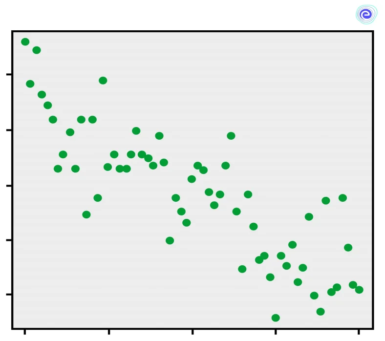
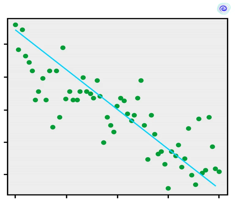
If this curve is a straight line, it is a case of linear regression, and the straight line is called the line of regression. Regression lines are the lines of best fit, so they try to cover as many points from the scatter diagram as possible. These lines express the average relationship between variables. In linear regression, we find the lines of regression by the concept curve fitting using the principle of least squares.

Why are there Two Lines of Regression?

The method of least squares minimises the sum of the squares of the errors from a specified value. Depending upon which variable we select as the dependent variable from \(x\) and \(y\), there can be two lines of regression.

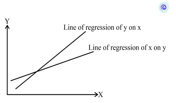
Line of Regression of \(x\) on \(y\)

We use this line to find the value of the dependent variable \(x\) for a given value of the independent variable \(y\). We use the least squares method to minimise the squares of the errors of the available values of \(y\) from the mean value of \(y\) i.e. \(\bar y\)

Line of Regression of \(y\) on \(x\)

We use this line to find the value of the dependent variable \(y\) for a given value of the independent variable \(x\). We use the method of least squares to minimise the squares of the errors of the available values of \(x\) from the mean value of \(x\) i.e. \(\bar x\)

Formula for Lines of Regression

The line of regression of \(x\) on \(y\) is given by the equation \((x – \bar x) = \frac{{r{\sigma _x}}}{{{\sigma _y}}}(y – \bar y)\).

The line of regression of \(y\) on \(x\) is given by the equation \((y – \bar y) = \frac{{r{\sigma _y}}}{{{\sigma _x}}}(x – \bar x)\).

Here,

\(\bar x =\) Mean of the values of \(x\)

\(\bar y =\) Mean of the values of \(y\)

\({\sigma _x} = \) Standard deviation of the values of \(x\) from \(\bar x \)

\({\sigma _y} = \) Standard deviation of the values of \(y\) from \(\bar y\)

\(r =\) Correlation coefficient

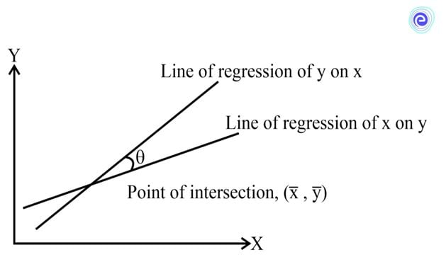
According to these formulas, we can see that both these lines pass through the point \((\bar x,\bar y)\). Thus, this is the point of intersection of these two lines.

Angle Between the Two Lines of Regression

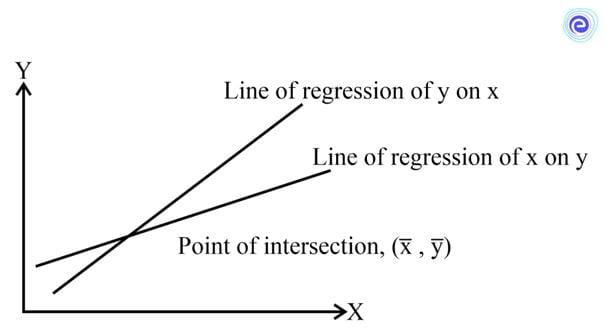
We have seen that the two lines of regression intersect at the point \((\bar x,\bar y)\). Therefore, for a correlation that is not perfect, the two lines will be at an angle \((\theta )\) to each other.

The line of regression of \(x\) on \(y\) is given by the equation \((x – \bar x) = \frac{{r{\sigma _x}}}{{{\sigma _y}}}(y – \bar y)\)

Let the slope of this line be \({m_1}\).

We can rewrite the line equation as \((y – \bar y) = \frac{{{\sigma _y}}}{{r{\sigma _x}}}(x – \bar x)\)

When we compare this with the standard line equation, \(y = mx + c\), we get

\({m_1} = \frac{{{\sigma _y}}}{{r{\sigma _x}}}\)

Similarly, the line of regression of \(y\) on \(x\) is given by the equation

\((y – \bar y) = \frac{{r{\sigma _y}}}{{{\sigma _x}}}(x – \bar x)\)

Here, let the slope of this line be \({m_2}\).

When we compare this with the standard line equation, \(y = mx + c\), we get

\({m_2} = \frac{{r{\sigma _y}}}{{{\sigma _x}}}\)

For two intersecting lines with slopes \({m_1}\) and \({m_2}\), the angle between these two lines, \(\theta \), can be found by the formula,

\(\tan \theta = \left| {\frac{{{m_1} – {m_2}}}{{1 + {m_1}{m_2}}}} \right|\)

\( \Rightarrow \tan \theta = \left| {\frac{{\frac{{{\sigma _y}}}{{r{\sigma _x}}} – \frac{{r{\sigma _y}}}{{{\sigma _x}}}}}{{1 + \frac{{{\sigma _y}}}{{r{\sigma _x}}} \times \frac{{r{\sigma _y}}}{{{\sigma _x}}}}}} \right|\)

\( \Rightarrow \tan \theta = \left| {\frac{{\frac{{{\sigma y}}}{{{\sigma _x}}}\left( {\frac{1}{r} – r} \right)}}{{1 + \frac{{{\sigma ^2}}}{{{\sigma {{x^2}}}}}}}} \right|\)

\( \Rightarrow \tan \theta = \left| {\frac{{{\sigma _y}}}{{{\sigma _x}}}\left( {\frac{{1 – {r^2}}}{r}} \right) \times \frac{{\sigma _x^2}}{{\sigma _x^2 + \sigma _y^2}}} \right|\)

\(\therefore \tan \theta = \left| {\left( {\frac{{1 – {r^2}}}{r}} \right)\frac{{{\sigma_x}{\sigma _y}}}{{{\sigma {{x^2} + \sigma _y^2}}}}} \right|\)

\( \Rightarrow \theta = {\tan ^{ – 1}}\left| {\left( {\frac{{1 – {r^2}}}{r}} \right)\frac{{{\sigma _x}{\sigma _y}}}{{\sigma _x^2 + \sigma _y^2}}} \right|\)

PRACTICE EXAM QUESTIONS AT EMBIBE

Type of Correlation and Angle of Regression

Following are the different types of Correlation and Angle of Regression

1. If we substitute \(r=0\) in the equation of \(\theta \) we get,

\(\theta = {\tan ^{ – 1}}\left| {\left( {\frac{{1 – {0^2}}}{0}} \right)\frac{{{\sigma_x}{\sigma _y}}}{{{\sigma_x^2 + \sigma _y^2}}}} \right|\)

\( \Rightarrow \theta = {\tan ^{ – 1}}\) (not defined)

\(\therefore \theta = \frac{\pi }{2}\)

It means that when \(r=0\), the angle between the lines of regression is \(\theta = \frac{\pi }{2}\).

\(r=0\) means the variables \(x\) and \(y\) have no correlation.

Thus, for uncorrelated variables \(x\) and \(y\), the lines of regression are perpendicular to each other.

2. If we substitute \(r = \pm 1\) in the equation of \(\theta \) we get,

\(\theta = {\tan ^{ – 1}}\left| {\left[ {\frac{{1 – {{( \pm 1)}^2}}}{{ \pm 1}}} \right]\frac{{{\sigma _x}{\sigma _y}}}{{\sigma _x^2 + \sigma _y^2}}} \right|\)

\( \Rightarrow \theta = {\tan ^{ – 1}}(0)\)

\(\therefore \theta = 0\) or \(\theta = \pi \)

It means that when \(r = \pm 1\), the angle between the lines of regression is \(\theta = 0\) or \(\theta = \pi \).

\(r = \pm 1\) means the variables have a perfect positive or perfect negative correlation.

Thus, for perfectly correlated (positive or negative) variables \(x\) and \(y\), the lines of regression are coincident.

3. The modulus\((||)\) in the formula of \(\theta \) indicates that it can take two values.

For a single value of \(r > 0\),

• \({\tan ^{ – 1}}\left( {\frac{{1 – {r^2}}}{r}} \right)\frac{{{\sigma _x}{\sigma _y}}}{{\sigma _x^2 + \sigma _y^2}}\) will give the acute angle between the two lines of regression, i.e., \(0 < \theta < \frac{\pi }{2}\).
• \({\tan ^{ – 1}}\left( {\frac{{{r^2} – 1}}{r}} \right)\frac{{{\sigma _x}{\sigma _y}}}{{\sigma _x^2 + \sigma _y^2}}\) will give the obtuse angle between the two lines of regression, i.e., \(\frac{\pi }{2} < \theta < \pi \).

4. As the angle between the two lines of regression decreases from \(\frac{\pi }{2}\) to \(0\), the correlation between the variables increases from \(0\) to \(1\).

5. As the angle between the two lines of regression increases from \(\frac{\pi }{2}\) to \(\pi \), the correlation between the variables increases from \(0\) to \(-1\).

Solved Examples – Angle Between Two Lines of Regression

Below are a few solved examples that can help in getting a better idea.

Q.1. For two variables, \(x\) and \(y\), the correlation coefficient is \(0.5\). The acute angle between the two lines of regression is \({\tan ^{ – 1}}\frac{3}{5}\). Show that \({\sigma _x} = \frac{1}{2}{\sigma _y}\).
Ans: Correlation coefficient, \(r=0.5\)

Angle between the two lines of regression, \(\theta = {\tan ^{ – 1}}\frac{3}{5}\)

Substituting these values in the equation of \(\theta \),

\(\theta = {\tan ^{ – 1}}\left| {\left( {\frac{{1 – {r^2}}}{r}} \right)\frac{{{\sigma _x}{\sigma _y}}}{{\sigma _x^2 + \sigma _y^2}}} \right|\)

Since, the angle given is acute, we can write

\(\theta = {\tan ^{ – 1}}\left( {\frac{{1 – {r^2}}}{r}} \right)\frac{{{\sigma _x}{\sigma _y}}}{{\sigma _x^2 + \sigma _y^2}}\)

\(\therefore {\tan ^{ – 1}}\frac{3}{5} = {\tan ^{ – 1}}\left( {\frac{{1 – {{0.5}^2}}}{{0.5}}} \right)\frac{{{\sigma _x}{\sigma _y}}}{{\sigma _x^2 + \sigma _y^2}}\)

\( \Rightarrow \frac{3}{5} = \left( {\frac{{1 – {{0.5}^2}}}{{0.5}}} \right)\frac{{{\sigma _x}{\sigma _y}}}{{\sigma _x^2 + \sigma _y^2}}\)

\( \Rightarrow \frac{3}{5} = \left( {\frac{{1 – 0.25}}{{0.5}}} \right)\frac{{{\sigma_x}{\sigma _y}}}{{\sigma _x^2 + {\sigma_y^2}}}\)

\( \Rightarrow \frac{3}{5} = \left( {\frac{{0.75}}{{0.5}}} \right)\frac{{{\sigma _x}{\sigma _y}}}{{\sigma _x^2 + \sigma _y^2}}\)

\( \Rightarrow \frac{3}{5} = \left( {\frac{3}{2}} \right)\frac{{{\sigma_x}{\sigma _y}}}{{{\sigma_x^2 + \sigma _y^2}}}\)

\( \Rightarrow 2\left( {\sigma _x^2 + \sigma _y^2} \right) = 5\left( {{\sigma _x}{\sigma _y}} \right)\)

\( \Rightarrow 2\sigma _x^2 – 5{\sigma _x}{\sigma _y} + 2\sigma _y^2 = 0\)

\( \Rightarrow 2{\sigma _x}^2 – 4{\sigma _x}{\sigma _y} – {\sigma _x}{\sigma _y} + 2{\sigma _y}^2 = 0\)

\( \Rightarrow 2{\sigma _x}\left( {{\sigma _x} – 2{\sigma _y}} \right) – {\sigma _y}\left( {{\sigma _x} – 2{\sigma _y}} \right) = 0\)

\( \Rightarrow \left( {{\sigma _x} – 2{\sigma _y}} \right)\left( {2{\sigma _x} – {\sigma _y}} \right) = 0\)

\( \Rightarrow \left( {{\sigma _x} – 2{\sigma _y}} \right) = 0\) or \(\left( {2{\sigma _x} – {\sigma _y}} \right) = 0\)

\( \Rightarrow \left( {2{\sigma _x} – {\sigma _y}} \right) = 0\)

\(\therefore {\sigma _x} = \frac{1}{2}{\sigma _y}\)

Q.2. For two variables, \(x\) and \(y\), regression coefficients are \({b_{xy}} = 0.4\) and \({b_{yx}} = 1.6\). If \(\theta \) is the angle between the two regression lines, then find the value of \(\theta \).
Ans: We know that,

\(\tan \theta = \left| {\left( {\frac{{1 – {r^2}}}{r}} \right)\frac{{{\sigma _x}{\sigma _y}}}{{\sigma _x^2 + \sigma _y^2}}} \right|\)

\( \Rightarrow \tan \theta = \left| {\left( {\frac{{1 – {r^2}}}{r}} \right)\frac{1}{{\frac{{{\sigma _x^2 + \sigma _y^2}}}{{{\sigma _x}{\sigma _y}}}}}} \right|\)

\( \Rightarrow \tan \theta = \left| {\left( {\frac{{1 – {r^2}}}{r}} \right)\frac{1}{{\frac{{{\sigma _x^2}}}{{{\sigma _x}{\sigma _y}}} + \frac{{{\sigma _y^2}}}{{{\sigma _x}{\sigma _y}}}}}} \right|\)

\( \Rightarrow \tan \theta = \left| {\left( {\frac{{1 – {r^2}}}{r}} \right)\frac{1}{{\frac{{{\sigma _x}}}{{{\sigma _y}}} + \frac{{{\sigma _y}}}{{{\sigma _x}}}}}} \right|\)

\(\therefore \tan \theta = \left| {\frac{{1 – {r^2}}}{{r\frac{{{\sigma _x}}}{{{\sigma _y}}} + r\frac{{{\sigma _y}}}{{{\sigma _x}}}}}} \right|\)

Now,

\(r\frac{{{\sigma_x}}}{{{\sigma _y}}} = {b_{xy}}\)

\(r\frac{{{\sigma_y}}}{{{\sigma _x}}} = {b_{yx}}\)

\({r^2} = {b_{xy}}{b_{yx}}\)

\(\therefore \tan \theta = \left| {\frac{{1 – {b_{xy}}{b_{yx}}}}{{{b_{xy}} + {b_{yx}}}}} \right|\)

This is one more formula for the angle between two lines of regression.

\(\therefore \tan \theta = \left| {\frac{{1 – 0.4 \times 1.6}}{{0.4 + 1.6}}} \right|\)

\( \Rightarrow \tan \theta = \left| {\frac{{1 – 0.64}}{{2.0}}} \right|\)

\( \Rightarrow \tan \theta = \left| {\frac{{0.36}}{{2.0}}} \right|\)

\(\therefore \tan \theta = |0.18|\)

Q.3. If the standard deviation of \(y\) is twice the standard deviation of \(x\), find the tangent of the acute angle between the two lines of regression if the correlation coefficient is \(0.25\).
Ans: Standard deviation of \(y = 2 \times ({\rm{Standard}}\,{\rm{deviation}}\,{\rm{of}}\,x)\)

\(\therefore {\sigma _y} = 2{\sigma _x}\)

Correlation coefficient, \(r=0.25\)

We know that for the acute angle between the two lines of regression,

\(\tan \theta = \left( {\frac{{1 – {r^2}}}{r}} \right)\frac{{{\sigma _x}{\sigma _y}}}{{\sigma _x^2 + \sigma _y^2}}\)

\( \Rightarrow \tan \theta = \left( {\frac{{1 – {{0.25}^2}}}{{0.25}}} \right)\frac{{{\sigma _x}\left( {2{\sigma _x}} \right)}}{{\sigma _x^2 + {{\left( {2{\sigma _x}} \right)}^2}}}\)

\( \Rightarrow \tan \theta = \left( {\frac{{1 – 0.0625}}{{0.25}}} \right)\frac{{2\sigma _x^2}}{{\sigma _x^2 + 4\sigma _x^2}}\)

\( \Rightarrow \tan \theta = \frac{{0.9375}}{{0.25}} \times \frac{2}{5}\)

\(\therefore \tan \theta = 1.5\)

Q.4. The regression lines of \(x\) on \(y\) and \(y\) on \(x\) are \(5x – y = 6\) and \(2x – 3y = – 8\), respectively. Find the angle between these lines.
Ans: Line of regression of \(x\) on \(y\)

\(5x – y = 6\)

\( \Rightarrow 5x = y + 6\)

\( \Rightarrow x = \frac{{y + 6}}{5}\)

\( \Rightarrow x = 0.2y + 1.2\)

\(\therefore {b_{xy}} = 0.2\)

Line of regression of \(y\) on \(x\)

\(2x – 3y = – 8\)

\( \Rightarrow – 3y = – 2x – 8\)

\( \Rightarrow y = \frac{{ – 2x – 8}}{{ – 3}}\)

\( \Rightarrow y = \frac{2}{3}x + \frac{8}{3}\)

\(\therefore {b_{yx}} = \frac{2}{3}\)

Angle between the two lines of regression,

\(\theta = {\tan ^{ – 1}}\left| {\frac{{1 – (0.2)\left( {\frac{2}{3}} \right)}}{{0.2 + \frac{2}{3}}}} \right|\)

\( \Rightarrow \theta = {\tan ^{ – 1}}\left| {\frac{{\frac{{3 – 0.4}}{3}}}{{\frac{{0.6 + 2}}{3}}}} \right|\)

\( \Rightarrow \theta = {\tan ^{ – 1}}\left| {\frac{{3 – 0.4}}{{0.6 + 2}}} \right|\)

\( \Rightarrow \theta = {\tan ^{ – 1}}\left| {\frac{{2.6}}{{2.6}}} \right|\)

\( \Rightarrow \theta = {\tan ^{ – 1}}|1|\)

\(\therefore \theta = \frac{\pi }{4}\)

This is the acute angle between the two lines of regression.

Q.5. The two lines of regression are \(6x + 15y = 27\) and \(6x + 3y = 15\). Calculate the angle between the two lines of regression.
Ans: We do not know which of these lines is the line of regression of \(x\) on \(y\) and the line of regression of \(y\) on \(x\).

Assume that the line of regression of \(x\) on \(y\) is \(6x + 15y = 27\), and the line of regression of \(y\) on \(x\) is \(6x+3y=15\).

We now represent these equations in proper form.

Line of regression of \(x\) on \(y\)

\(6x + 15y = 27\)

\( \Rightarrow 6x = – 15y + 27\)

\( \Rightarrow x = \frac{{ – 15y + 27}}{6}\)

\( \Rightarrow x = – 1.5y + 4.5\)

\(\therefore {b_{xy}} = – 1.5\)

Line of regression of \(y\) on \(x\)

\(6x + 3y = 15\)

\( \Rightarrow 3y = – 6x + 15\)

\( \Rightarrow y = \frac{{ – 6x + 15}}{3}\)

\( \Rightarrow y = – 2x + 5\)

\(\therefore {b_{yx}} = – 2\)

According to this assumption, \({b_{xy}} = – 1.5\) and \({b_{yx}} = – 2\) 

We know that,

\(r = \sqrt {{b_{xy}}{b_{yx}}} \)

\(\therefore r = \sqrt { – 1.5 \times – 2} \)

\(\therefore r = \sqrt 3 \)

This assumption gives a value of \(r>1\), which is not possible. It means our assumption is incorrect.

Thus,

\(6x + 15y = 27\) – Line of regression of \(y\) on \(x\) and \(6x + 3y = 15\) – Line of regression of \(x\) on \(y\)

Line of regression of \(y\) on \(x\)

\(6x + 15y = 27\)

\(\therefore 15y = – 6x + 27\)

\(\therefore y = \frac{{ – 6x + 27}}{{15}}\)

\(\therefore y = – 0.4x + 1.8\)

\(\therefore {b_{yx}} = – 0.4\)

Line of regression of \(x\) on \(y\)

\(6x + 3y = 15\)

\(\therefore 6x = – 3y + 15\)

\(\therefore x = \frac{{ – 3y + 15}}{6}\)

\(\therefore x = – 0.5y + 2.5\)

\(\therefore {b_{xy}} = – 0.5\)

Angle between the two lines of regression,

\(\theta = {\tan ^{ – 1}}\left| {\frac{{1 – {b_{xy}}{b_{yx}}}}{{{b_{xy}} + {b_{yx}}}}} \right|\)

\(\therefore \theta = {\tan ^{ – 1}}\left| {\frac{{1 – ( – 0.5)( – 0.4)}}{{( – 0.5) + ( – 0.4)}}} \right|\)

\(\therefore \theta = {\tan ^{ – 1}}\left| {\frac{{1 – 0.2}}{{ – 0.9}}} \right|\)

\(\therefore \theta = {\tan ^{ – 1}}\left| {\frac{{0.8}}{{ – 0.9}}} \right|\)

\(\therefore \theta = {\tan ^{ – 1}}\left| {\frac{8}{{ – 9}}} \right|\)

Summary

There are two lines of regression, each trying to minimise the deviations of \(x\) and \(y\) from their means by the method of least squares. The two lines of regression intersect at the point whose coordinates give the means of both the variables, i.e. \((\bar x,\bar y)\). The formula for the angle between the two lines of regression is \(\theta = {\tan ^{ – 1}}\left| {\left( {\frac{{1 – {r^2}}}{r}} \right)\frac{{{\sigma _x}{\sigma _y}}}{{\sigma _x^2 + \sigma _y^2}}} \right|\). When the angle between the two lines of regression is \(0\) or \(\pi \) then there is a perfect correlation between the two variables. When the angle between the two lines of regression is \(\frac{\pi }{2}\) then there is no correlation between the two variables. Thus, the angle between the two lines of regression is a connecting link between regression and correlation.

FAQs on Angle Between Two Lines of Regression

Students might be having many questions with respect to the Angle Between Two Lines of Regression. Here are a few commonly asked questions and answers.

Q.1. How do you find the angle between two regression lines?
Ans: You can find the angle between the two lines of regression by using the formula
\(\theta = {\tan ^{ – 1}}\left| {\left( {\frac{{1 – {r^2}}}{r}} \right)\frac{{{\sigma _x}{\sigma _y}}}{{\sigma _x^2 + \sigma _y^2}}} \right|\)
Here,
\({\sigma _x} = \) Standard deviation of the values of \(x\) from \(\bar x\)
\({\sigma _y} = \) Standard deviation of the values of \(y\) from \(\bar y\)
\(r=\) Correlation coefficient

Q.2. What are the two lines of regression?
Ans: The two lines of regressions are a line of regression of \(x\) on \(y\) and a line of regression of \(y\) on \(x\).

• Line of regression of \(x\) on \(y\) – It establishes a relationship between \(x\) and \(y\). It is used to find the unknown value of the dependent variable \(x\) for a known value of the independent variable \(y\).
• Line of regression of \(y\) on \(x\) – It establishes a relationship between \(y\) and \(x\). It is used to find the unknown value of the dependent variable \(y\) for a known value of the independent variable \(x\).

Q.3. Under what condition will the angle between two regression lines become zero?
Ans: The angle between the two regression lines becomes zero when the two variables are in perfect correlation, either positive or negative.

Q.4. When the correlation coefficient increases from \(0\) to \(1\), how does the angle between the regression lines diminish?
Ans: When the correlation coefficient increases from \(0\) to \(1\), the angle between the regression lines diminishes from \(\frac{\pi }{2}\) to \(0\).

Q.5. Why there are two regression lines? Write the properties of regression lines.
Ans: There are two lines of regression each trying to minimise the squares of deviations of \(x\) and \(y\) from their means by the method of least squares.
Line of regression of \(x\) on \(y\) – It minimises the deviations of squares of values of \(x\) from its mean \(\bar x\) parallel to the \(X\)-axis.
Line of regression of \(y\) on \(x\) – It minimises the deviations of squares of values of \(y\) from its mean \(\bar y\) parallel to the \(Y\)-axis.

ATTEMPT MOCK TESTS ON EMBIBE

We hope this information about the Angle Between Two Lines of Regression has been helpful. If you have any doubts, comment in the section below, and we will get back to you soon.