Approximations: An estimation or approximation is a reasonable guess about the measure of quantity. It is the process of making guesses without any actual measurement or calculation. Approximations are sometimes important as we do not have all the facts or are pressed for time. Approximation theory is a theoretical study of methods that use numerical approximation for problems in mathematical analysis.

In reality, it is typically the form of computation of problems in various scientific disciplines and the application of computer simulation. Numerical algorithms in approximation theory have been a significant research thrust with numerous applications. The approximation has its uses in daily life as well. For example, when we cook, we use an approximation for adding salt and spices.

What are Errors?

Let a function \(y = f\left( x \right)\) be defined. If \(\Delta x\) is the error that occurred while calculating \(x\), we may also get an error in the calculation of \(y\), i.e., \(f(x)\). The correct value of \(y\) should have been \(y = (x + \Delta x)\). But the value that we have obtained because of the error in the calculation of \(x\) will be \(y = f(x)\). Therefore \(f(x + \Delta x) – f(x)\) will be the error in the calculation of \(y\) and is denoted \(\Delta y\).

Types of Errors

The following are different types of Errors

1. Absolute errors: It is the deviation of measured value of physical quantity from its actual value i.e., error \( = \Delta y = f\left( {x + \;\Delta x} \right) – f\left( x \right)\)
2. Relative errors: It is the ratio of error to the total quantity measured e.g. \(\frac{{\delta y}}{y}\) where \(\delta y\) is absolute error and \(y\) is actual value.
3. Percentage errors: It is given by relative error \(\times 100\) i.e., \(\frac{{\delta y}}{y} \times 100\)
4. Maximum probable error: It is the error encountered in the final measured quantity assuming that all the errors occurring in the measurement of component quantities have same sign i.e., cumulative in nature e.g. if \(z = f(x) + f(y)\) then maximum probable error in \(z = \left| {error\;in\;f\left( x \right)} \right| + \left| {error\;in\;f\left( y \right)} \right|\).

Note: We must be careful to distinguish between derivatives and differentials. They are certainly not the same

When we write \(\frac {dy}{dx}\),  we are using a symbol, the derivative and when we write \(dy\), we denote a differential.

What is Approximation?

As the name suggests, the topic approximation is useful to find the approximate value of \(y = f(x)\) when a small change in \(x\) has occurred. For example, If we need to find the approximate value of \(y = \sqrt {0.0037}\) or \(y = \sqrt {64.2}\) etc.

What is Linear Approximation?

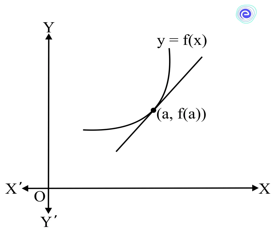
The linear approximation is nothing but the equation of a tangent line. The slope of a tangent which is drawn to a curve \(y = f(x)\) at a point \(x = a\) is its derivative at \(x = a\). i.e., the slope of a tangent line is \(f'(a)\) Thus, the linear approximation formula is an application of derivatives.

The linear approximation of a function is nothing but the approximate value of the function at a point using a line. Whenever we see a curve of a function and any point on it, we come to the concept of the tangent line.

If we can find the equation of the tangent at the given point, then we can find the approximated value of the function at any point that is very close to the given point using the equation of the tangent line. This concept is known as the linear approximation and since we are using the tangent line for it, it is also known as the tangent line approximation.

Formula for the Linear Approximations

The linear approximation formula is nothing but the equation of the tangent line. The equation of a tangent line that is drawn to the curve \(y = f(x)\) at the point \(x = a\) (or) \((a, f(a))\) using the point-slope form is:

\(L\left( x \right) = f\left( a \right) + f’\left( a \right)\left( {x – a} \right)\)

Where \(f'(a)\) is the slope of the tangent at \(x = a\).

Differential Calculus and Approximations

Now, let’s see the differentials used to approximate certain quantities. Let a function \(f\) in \(x\) be defined such that \(f:\;A\; \to B,\;\,A\; \subset \;B.\) Let \(y = f(x)\). Let the small increase in \(x\) is denoted by \(\Delta x\). If \(x\) increases by \(\Delta x\) then the corresponding \(y\) is increased by \(\Delta y = f\left( {x + \Delta x} \right) – f(x)\), as shown in the figure below.

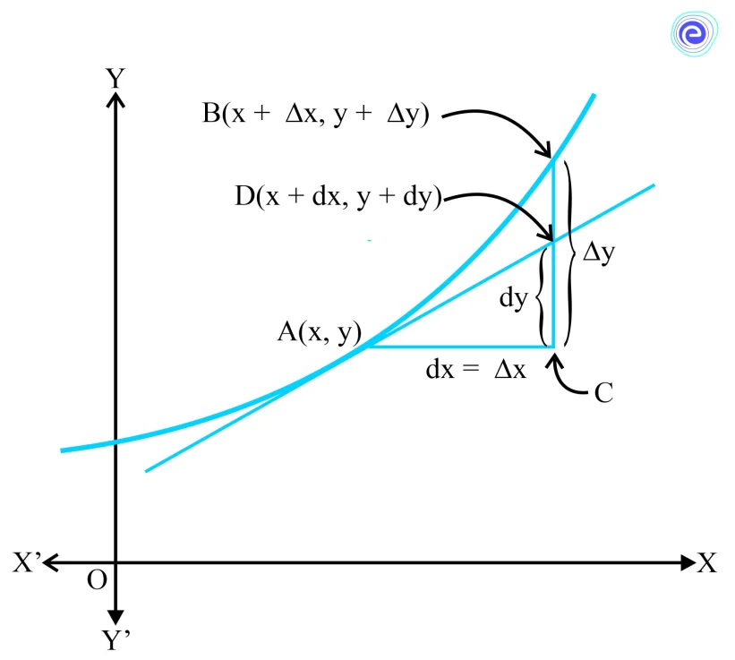
Based on the discussion, we can write the following points:

• The differential of \(x\) which is represented as \(dx\) is given by \(dx = \Delta x\).
• The differential of \(y\) which is represented as \(dy\) is given by \(dy = f’\;\left( x \right)dx = \left( {\frac{{dy}}{{dx}}} \right)\Delta x\).

If the differential of \(x\) or \(dx = \Delta x\) is comparatively negligible in comparison to \(x\) then \(dy\) is a good approximation of \(\Delta y\) and \(dy\; \approx \;\Delta y.\)

Note: The differential of the independent variable is equal to the increase in the variable, but the differential of the dependent variable is not equal to the increase of the variable.

Approximations Algorithm

Following are the steps of the Approximations Algorithm:

Step 1: Define a functional relationship between the independent variable \(x\) and dependent variable \(y\) by observing the given expression.

For example, if we have to find the approximate value of the square root or cube root of a number, then we define \(y = {x^{\frac{1}{2}}}\) or \({x^{\frac{1}{3}}}\) respectively. Similarly, if we have to find the approximate value of logarithmic of a given number, then we consider \(y = \log x\)

Step 2: Choose a value of \(x\) nearest to the value, at which we have to find \(y\) in such a way that either \(y\) is given for the chosen \(x\) or \(y\) can be easily computed for the chosen value of \(x\).

For example, if we have to find an approximate value of \({\left( {127} \right)^{\frac{1}{3}}}\) we take \(x\) as \(125\) because the cube root of \(125\) can be easily calculated.

Step 3: Denote the value of \(x\) at which we have to find \(y\) by \(x + \Delta x\)

Step 4: Find \(\Delta x\) and assume that \(dx = \Delta x\)

Step 5: Find \(\frac {dy}{dx}\) from the relation obtained in step 1.

Step 6: Find the value of \(\frac {dy}{dx}\) by putting the value of \(x\) chosen in step 2.
\(\because \,f’\left( x \right) = \mathop {\lim }\limits_{\delta x \to 0} \frac{{f\left( {x + \delta x} \right) – f\left( x \right)}}{{\delta x}}\)

Step 7: Find \(dy\) by using the relation \(dy = \frac{{dy}}{{dx}}dx\)
i.e., \(\frac{{dy}}{{dx}} = \mathop {\lim }\limits_{\delta x \to 0} \frac{{\delta y}}{{\delta x}}\)

Step 8: Assume that \(\Delta y \cong dy\)

Step 9: Find the value of \(y\) by putting the value of \(x\) chosen in step 2 in the relation obtained in step 1.

Step 10: The approximate value of \(y\) is \(y + \Delta y\)
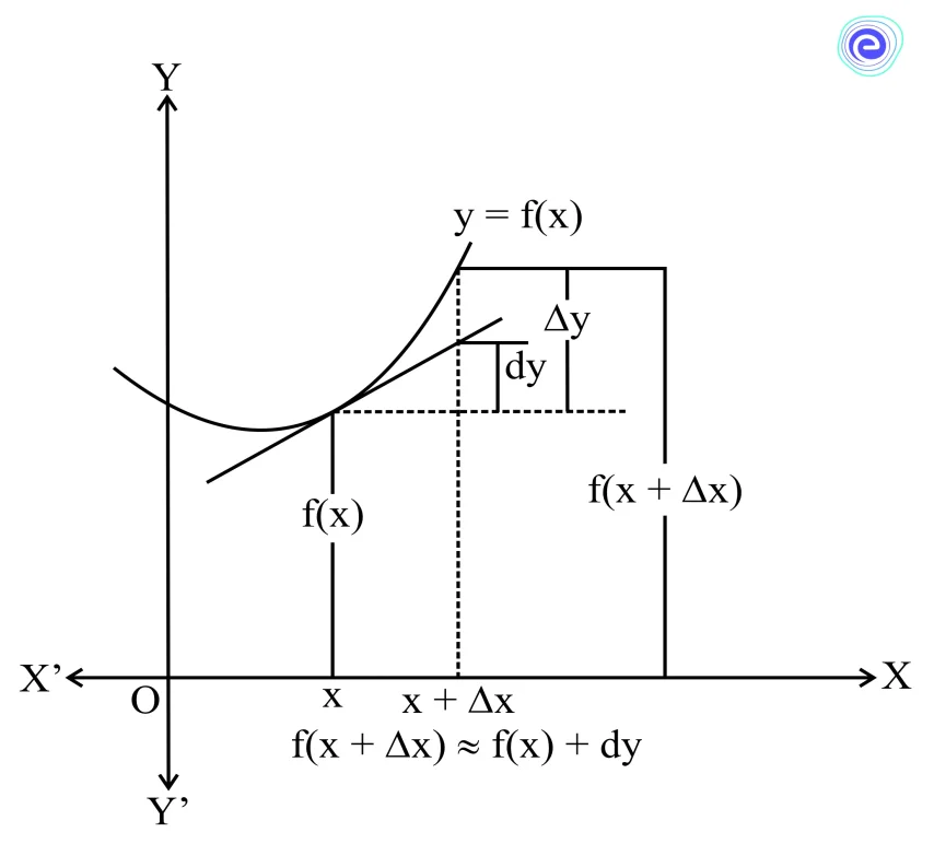
i.e., if \(\Delta x\) is very small w.r.t \(x\) then \(\frac{{dy}}{{dx}} \approx \frac{{\delta y}}{{\delta x}} \Rightarrow \delta y = \frac{{dy}}{{dx}}\delta x\)

\(\because \,f\left( {x + \delta x} \right) – f\left( x \right) = \frac{{dy}}{{dx}} \cdot \delta x\)

\(\Rightarrow f\left( {x + \delta x} \right) = f\left( x \right) + \frac{{dy}}{{dx}} \cdot \delta x\)

Solved Examples on Approximations

Below are a few solved examples that can help in getting a better idea.

Q.1. If there is an error of \(k\%\) in measuring the edge of a cube, then find the percent error in estimating its volume.
Ans: volume of a cube \(= v = x^3\) and the percent error in measuring \(x = \frac {dx}{x} \times 100\)
The percent error in measuring volume \(= \frac {dv}{v} \times 100\)
Now, \(\frac{{dv}}{{dx}} = 3{x^2}\; \Rightarrow dv = 3{x^2}dx\)
\(\therefore \,\frac{{dv}}{v} = \frac{{3{x^2}dx}}{{{x^3}}} = \frac{{3dx}}{x}\)
\(\therefore \,\frac{{dv}}{v} \times 100 = 3\frac{{dx}}{x} \times 100 = 3k\%\).

Q.2. Find the approximate value of \((0.007)^{\frac {1}{3}}\).
Ans: Let \(f\left( x \right) = {x^{\frac{1}{3}}}\; \Rightarrow f’\left( x \right) = \frac{1}{3}{x^{ – \frac{2}{3}}}\)
Now \(f(x + \Delta x) – f(x) = f'(x) \cdot \Delta x = \frac{{\Delta x}}{{3\left( {{x^{\frac{2}{3}}}} \right)}}\)
We may write \(0.007 = 0.008 – 0.001\), taking \(x = 0.008\) and \(dx = – 0.001\)
We have \(f(0.007) – f(0.008) = – \frac{{0.001}}{{3{{(0.008)}^{ – \frac{2}{3}}}}}\)
\(\Rightarrow f(0.007) – {(0.008)^{\frac{1}{3}}} = – \frac{{0.001}}{{3{{(0.2)}^2}}}\)
\(\Rightarrow f(0.007) = 0.2 – \frac{{0.001}}{{3(0.04)}} = 0.2 – \frac{1}{{120}} = 23/120\)
Hence, \({(0.007)^{\frac{1}{3}}} = \frac{{23}}{{120}}\).

Q.3. Find the approximate value of \(f(3.02)\), where \(f(x) = 3x^2 + 5x + 3\)
Ans: Let \(x = 3\) and \(x + \Delta x = 3.02\), then \(\Delta x = 0.02\)
We have \(f\left( x \right) = 3{x^2} + 5x + 3\)
\(\Rightarrow f\left( 3 \right) = 3 \times {3^2} + 5 \times 3 + 3 = 45\)
Now \(y = f(x)\)
\(\Rightarrow \Delta y = \frac{{dy}}{{dx}}\Delta x\)
\(\Rightarrow \Delta y = \left( {6x + 5} \right)\Delta x = \left( {6\left( 3 \right) + 5} \right) \cdot \left( {0.02} \right) = 0.46\)
\(\left[ {\because \,y = f\left( x \right) = 3{x^2} + 5x + 3\; \Rightarrow \frac{{dy}}{{dx}} = 6x + 5\;} \right]\)
\(\therefore \,f\left( {3.02} \right) = f\left( {x + \Delta x} \right) = y + \Delta y = 45 + 0.46 = 45.46\)
Hence, the approximate value of \(f(3.02)\) is \(45.46\).

Q.4. The pressure \(p\) and volume \(v\) of gas is given by the relation \(pv^{1.4} = const\). Find the percentage error in \(p\) corresponding to a decrease of \(1.2\%\) in \(v\).
Ans: We have, \(pv^{1.4} = k (constant)\)
\(\Rightarrow \log p + 1.4\log v = \log k\)
\(\Rightarrow \frac{1}{p}\frac{{dp}}{{dv}} + \frac{{1.4}}{v} = 0 \Rightarrow \frac{{dp}}{{dv}} = – \frac{{1.4p}}{v}\)
Now, \(\Delta p = \frac{{dp}}{{dv}}\Delta v\)
\(\Rightarrow \Delta p = – \frac{{1.4p}}{v}\Delta v \Rightarrow \frac{{\Delta p}}{p} = – 1.4\frac{{\Delta v}}{v}\)
\(\Rightarrow \frac{{\Delta p}}{p} \times 100 = – 1.4\left( {\frac{{\Delta v}}{v} \times 100} \right)\)
\(\Rightarrow \frac{{\Delta p}}{p} \times 100 = – 1.4( – 1.2) = 0.7\,\left[ {\because \,\frac{{\Delta v}}{v} \times 100 = 1.2,\;{\text{given}}} \right]\).

Q.5. Find the linear approximation of function \(f(x) = x^3 – x\) around \(x = 3\).
Ans: The linear approximation is the same thing as the tangent line. The equation for the linear approximation around \(x = 3\) is \(L3\left( x \right) = f’\left( 3 \right)\left( {x – 3} \right) + f\left( 3 \right).\)
The derivative of \(f\) is \(f’\left( x \right) = 3{x^2} – 1\)
Therefore \(f(3) = 24\) and \(f'(3) = 26\) and the linear approximation is
\({L_3}\left( x \right) = 26\left( {x – 3} \right) + 24 = 26x – 54\).

Summary

Let a function \(y = f(x)\) be defined and if \(\Delta x\) is the error that occurred while calculating \(x\), then we may also get an error in the calculation of \(y\) i.e., \(f(x)\). There are four types of error (i) Absolute error, (ii) Relative error, (iii) Percentage errors, and (iv) Maximum probable error. As the name suggests, the topic approximations are useful to find the approximate value of \(y = f(x)\) when a small change in \(x\) has occurred.

The linear approximation of a function is nothing but the approximate value of the function at a point using a line. \(L\left( x \right) = f\left( a \right) + f’\left( a \right)\left( {x – a} \right)\) is the formula for linear approximation. Let \(y = f(x)\). Let the small increase in \(x\) is denoted by \(\Delta x\). If \(x\) increases by \(\Delta x\) then the corresponding \(y\) is increased by \(\Delta y = f(x + \Delta x) – f(x)\).

FAQs on Approximations

Students might be having many questions regarding Approximations. Here are a few commonly asked questions and answers.

Q.1. What is the example of Approximation?
Ans: As the name suggests, the topic approximations are useful to find the approximate value of \(y = f(x)\) when a small change in \(x\) has occurred. For example, if we have to find an approximate value of \((127)^{\frac {1}{3}}\) we take \(x\) as \(125\) because the cube root of \(125\) can be easily calculated.

Q.2. What is an Approximation in Math?
Ans: An approximation is something similar, but not exactly equal, to something else. A number can be approximated by rounding. A calculation can be approximated by rounding the values before performing the operations.

Q.3. How many types of Approximation are there?
Ans: There are two types of approximation algorithms that have been used for this purpose: sampling algorithms, such as importance sampling and Markov chain Monte Carlo, and variational algorithms, such as mean-field approximations and assumed density filtering

Q.4. What is small angle approximation?
Ans: Following are the small angle approximation for the basic trigonometric function, and it is valid when \(\theta \approx 0\):
\(\sin \theta \approx \theta \), \(\cos \theta \approx 1 – \frac{{{\theta ^2}}}{2} \approx 1\), \(\tan \theta \approx \theta \).

Q.5. What is linear approximation?
Ans: The linear approximation of a function is nothing but the approximate value of the function at a point using a line. Whenever we see a curve of a function and any point on it, we come to the concept of the tangent line. If we can find the equation of the tangent at the given point, then we can find the approximated value of the function at any point that is very close to the given point using the equation of the tangent line. This concept is known as the linear approximation and since we are using the tangent line for it, it is also known as the tangent line approximation.