Further Partition Values: Definition, Quartiles, Deciles, Percentile

Further Partition Values: The partition values have a wide range of applications in government policies to eradicate poverty and unemployment issues. Partition values are statistical measures for dividing a total number of distribution observations into a specified number of equal pieces. Quartiles, deciles, and percentiles are common partition values.

It is imperative to remember that the data should be sorted in ascending or descending order before the partition values are calculated. Quartiles divide data into four equal parts, deciles into \(10\) equal parts, and percentiles into one hundred equal parts. These partition values break down a more extensive distribution into smaller sections that are easier to measure, analyse, and understand.

Definition of Partition Values

The general definition of partition values is the magnitudes of those elements in an array that divide the number of items into some given number of equal pieces is known as partition values. These are the values of the items that divide the series into several pieces. Quartiles, quintiles, octiles, deciles, and percentiles are some such partition values in Statistics. These partition values give an overview of how the series is formed and are used to calculate dispersion and skewness.

Thus, partition values are the variate values dividing the total number of observations into equal parts. Whenever we have an observation that we want to divide, we can do so in a variety of ways.

• Quartiles are the values dividing the whole observations into four equal parts.
• Deciles are the variate values dividing the whole observations into \(10\) equal parts, so there are \(9\) deciles.
• Percentiles are the variate values dividing the entire observation into \(100\) equal parts, and hence, there are \(99\) percentiles.

Quartiles

We use the median when a single observation is divided into two equal portions. Quartiles are values that divide a particular set of observations into four equal parts using quartiles.

1. First \(25\%\) of observations
2. Next \(25\%\) of observations (up to median value)
3. Next \(25\%\) of the observations greater than the median
4. Next \(25\%\) of the observations

The data is divided into four equal parts by three quartiles.

• First Quartile \((Q_1)\)
• Second Quartile \((Q_2)\)
• Third Quartile \((Q_3)\)

Each component contains one-fourth of the data values. The first quartile \((Q_1)\) second quartile \((Q_2)\), and third quartile \((Q_3)\) are called the lower quartile, middle quartile (or median), and upper quartiles, respectively.

Quartiles for Ungrouped Data

First Quartile \((Q_1)\)

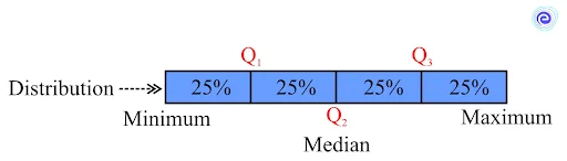
The first quartile \((Q_1)\) distinguishes the first one-fourth of the data from the upper three-fourths of the data, i.e., \(25\%\) of the data will fall below \((Q_1)\) and \(75\%\) will fall above it. The mathematical formula for \((Q_1)\) is given below, where N is the total number of observations in the data set.
\({Q_1} = 1 \times {\left( {\frac{{N + 1}}{4}} \right)^{th}}\) observation

Second Quartile \((Q_2)\)

The data is divided into two equal sections by the second quartile \((Q_2)\). It divides the initial half of the data from the second half of the data. \(50\%\) of the data falling below \((Q_2)\) and the other \(50\%\) falling above it. The median of the data is sometimes known as the second quartile \((Q_2)\).
\({Q_2} = 2 \times {\left( {\frac{{N + 1}}{4}} \right)^{th}}\) observation

Third Quartile \((Q_3)\)

The third quartile \((Q_3)\) divides the first three-quarters of the data from the last quarter. \(75\%\) of the data falling below \((Q_3)\) and \(25\%\) falling above it.
\({Q_3} = 3 \times {\left( {\frac{{N + 1}}{4}} \right)^{th}}\) observation

Steps to Calculate

The first quartile \((Q_1)\) of a distribution is equal to the median of the first half of the data set. The third quartile \((Q_3)\)  is equal to the median of the second half of the data set; the second quartile \((Q_2)\) of a distribution is equal to the median of the given data set.

• Step 1: Arrange the numbers in ascending or descending order.
• Step 2: Find the median of the given numbers.
• Step 3: Put parentheses around the numbers higher than the median.
• Step 4: Find the median of those numbers inside the parentheses. This is the value of the upper quartile.
• Step 5: Put parentheses around the numbers lower than the median.
• Step 6: Find the median of those numbers, which gives the value of the lower quartile.

Interquartile Range

The interquartile range (IQR) measures the middle \(50\%\) of the data.  It is the smallest of all statistical measures of dispersion and is calculated as the difference between the upper and lower quartiles.

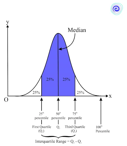
Interquartile range \(= Q_3 – Q_1\)
Where,

• \({Q_1} = 1 \times {\left( {\frac{{N + 1}}{4}} \right)^{th}}\) observation
• \({Q_1} = 3 \times {\left( {\frac{{N + 1}}{4}} \right)^{th}}\) observation

Quartiles for Grouped Data

The formula to calculate the \(i^{th}\) quartile is given below:
\({Q_i} = l + \left( {\frac{{\frac{{in}}{4} – {c^i}}}{f}} \right)h\)
Where,

• \(l\) is the lower class boundary of the class containing the \(i^{th}\) decile
• \(h\) is the width of the class containing \((Q_i)\)
• \(f\) is the frequency of the class containing
• \(n\) is the total number of frequencies \((Q_i)\)
• \(c^i\) is the cumulative frequency of the class immediately preceding to the class containing \((Q_i)\)

How to Calculate?

Following are the steps to calculate,

• Step 1: Add all the frequencies to get the value of \(n\).
• Step 2: Calculate the cumulative frequencies for all class intervals 
• Step 3: To obtain the \(i^{th}\) quartile \({(}i = 1, 2\) or \(3{)}\) find the value of \(\left( {\frac{{in}}{4}} \right)\)
• Step 4: The quartile belongs to the class with a cumulative frequency just above \(\left( {\frac{{in}}{4}} \right)\). Using the formula, determine the value of the \(i^{th}\) quartile.

What are Deciles?

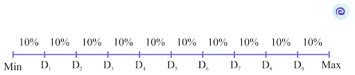
The partition values dividing data collection into \(10\) equal parts are called deciles. The first, second, third, ….. and ninth deciles are marked as \({{\text{D}}_1},\;{{\text{D}}_2},\;{{\text{D}}_3},\;{{\text{D}}_4},\; \ldots ..\;{{\text{D}}_9}\) and are referred to as \(1^{st}\) decile, \(2^{nd}\) decile, \(3^{rd}\) decile…., and \(9^{th}\) decile, respectively. For decile calculation, the data should be in ascending or descending order of magnitude.

Deciles for Ungrouped Data

• The first decile \(D_1\) is the point where \(10\%\) of the observations are below it and \(90\%\)of the observations are above it.
• The second decile \(D_2\) is the point where \(20\%\) of the observations are below it and \(80\%\) of the observations are above it.
• The \(9^{th}\) Decile \(D_9\), on the other hand, is the point where \(90\%\) of the observations are below it, and \(10\%\) are above it.
• The \(5^{th}\) decile \(D_5\) divides the data into two equal parts. So, the \(5^{th}\) decile \(D_5\) is the same as the median.
• The formula for the \(i^{th}\) decile \(D_i\) in mathematics is as follows:
  \({D_i} = i \times {\left( {\frac{{N + 1}}{{10}}} \right)^{th}}\)

Deciles for Grouped Data

The \(m^{th}\) decile for a grouped data is calculated by using the formula:
\({D_m} = l + \left( {\frac{{\frac{{mn}}{{10}} – {c^m}}}{f}} \right)h\)
Where,

• \(l\) is the lower class boundary of the class containing the \(m^{th}\) decile
• \(h\) is the width of the class containing \(D_m\)
• \(f\) is the frequency of the class containing \(D_m\)
• \(n\) is the total number of frequencies \(D_m\)
• \(c^m\) is the cumulative frequency of the class immediately preceding the class containing \(D_m\)

Percentiles

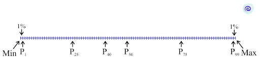
Percentiles divide a distribution into \(100\) equal portions, dividing the entire data set into \(100\) groups. Each percentile consists of \(1\%\) of data. The total of \(99\) percentiles are denoted by the letters \({{\text{P}}_1},\;{{\text{P}}_2},\;{{\text{P}}_3},\;{{\text{P}}_4},\; \ldots \ldots \ldots {{\text{P}}{99}}\) and are referred to as the \(1^{st}\) percentile, \(2^{nd}\) percentile,…., \(99^{th}\) percentile.

It should be mentioned that before calculating percentiles, the data should be sorted in ascending or descending order of magnitude.

Percentiles for Ungrouped Data

The \(k^{th}\) percentile in a data collection is the value that divides the data into two parts:

• The data in the lower half is made up of \(k\) percent of the total.
• The rest of the data is in the upper part, and it corresponds to \((100 – k)\) percent, where \(k\) can be any value between \(0\) and \(100\).

The median of the data, which divides the series into two equal portions, is equivalent to the \(50^{th}\) percentile. The formula for the \(i^{th}\) percentile \(P_i\) in mathematics is as follows:
\({P_i} = i \times {\left( {\frac{{N + 1}}{{100}}} \right)^{th}}\) observation

Percentile for Grouped Data

The \(k^{th}\) percentile for a groped data is calculated by using the formula:
\({P_k} = l + \left( {\frac{{\frac{{kn}}{{100}} – {c^k}}}{f}} \right)h\)
Where,

• \(l\) is the lower class boundary of the class containing the \(k^{th}\) percentile
• \(h\) is the width of the class containing \(P_k\)
• \(f\) is the frequencyof the class containing \(P_k\)
• \(n\) is the total number of frequencies \(P_k\)
• \(c^{k}\) is the cumulative frequency of the class immediately preceding the class containing \(P_k\)

Solved Examples – Further Partition Values

Below are a few solved examples that can help in getting a better idea.

Q.1. The marks of the Siva Ramakrishna in Mathematics examination is as follows:
\(70,\;66,\;48,\;64,\;59,\;74,\;51,\;40,\;62,\;77,\;60,\;33\)
Find the median marks by using the quartiles.
Ans:
Ascending order: \(33,\;40,\;48,\;51,\;59,\;60,\;62,\;64,\;66,\;70,\;74,\;77\)
\(\therefore\) Number of observations \((N) = 12\)
\({Q_1} = 2 \times {\left( {\frac{{N + 1}}{4}} \right)^{th}}\)
\({Q_2} = 2 \times {\left( {\frac{{12 + 1}}{4}} \right)^{th}} = {6.5^{th}}\) observation
\({Q_2} = {6^{th}}\) observation \(+ 0.5 \times {(}7^{th}\) observation – \(6^{th}\) observation\({)}\)
\(\therefore \,{Q_2} = 60 + 0.5 \times \left( {62 – 60} \right) = 61\)

Q.2. Find the \({6^{th}}\) decile for the data given below:
\(11,\;25,\;20,\;15,\;24,\;28,\;19,\;21\)
Ans:
Arrange the given data in ascending order as follows:
\(11,\;15,\;19,\;20,\;21,\;24,\;25,\;28\)
The formula to calculate the \({6^{th}}\) decile is given by
\({D_6} = 6 \times {\frac{{\left( {N + 1} \right)}}{{10}}^{th}}\) observation
\({D_6} = 6 \times {\frac{{\left( {8 + 1} \right)}}{{10}}^{th}}\) observation
\({D_6} = 6 \times {0.9^{th}} = {5.4^{th}}\) observation
\({D_6} = {5^{th}}\) observation \(+ 0.4 \times {(} {6^{th}}\) observation \(- {5^{th}}\) observation\({)}\)
\({D_6} = 21 + 0.4 \times \left( {24 – 21} \right)\)
\( = 21 + 0.4 \times 3 = 21 + 1.2\)
\(\therefore \,{D_6} = 22.2\)

Q.3. The following is the monthly income (in \(1000\)) of \(8\) factory workers. Find out how much \(P_{30}\) is worth.
\(10,\;14,\;36,\;25,\;15,\;21,\;29,\;17\)
Ans:
Ascending order: \(10,\;14,\;15,\;17,\;21,\;25,\;29,\;36\)
Number of observations \((N) = 8\)
The formula to calculate \(P_{30}\) is given by
\({P_{30}} = 30 \times {\left( {\frac{{N + 1}}{{100}}} \right)^{th}}\) observation
\({P_{30}} = 30 \times {\left( {\frac{{9 + 1}}{{100}}} \right)^{th}}\) observation
\({P_{30}} = {2.7^{th}}\) observation
\({P_{30}} = {2^{nd}}\) observation \(+ 0.7 \times {(} 3^{rd}\) observation \(- 2^{nd}\) observation\({)}\)
\({P_{30}} = 14 + 0.7 \times \left( {15 – 14} \right)\)
\({P_{30}} = 14 + 0.7\)
\(\therefore \,{P_{30}} = 14.7\)

Q.4. Compute \(Q_3\) for the wages in the given data.

Ans:

From the data, \(n = 86\)
\(\frac{{n3}}{4} = \frac{{86 \times 3}}{4} = 64.5\)
The class \(38 – 40\) has a cumulative frequency \(72\), which is greater than \(\frac{{n3}}{4} = 64.5\)
The \(3^{rd}\) quartile class is \(38 – 40\)
So,
\(l = 38\)
\(h = 2\)
\(f = 12\)
\(cf = 60\)
So, \({Q_i} = l + \left( {\frac{{\frac{{in}}{4} – {c^i}}}{f}} \right)h\)
\({Q_3} = l + \left( {\frac{{\frac{{3n}}{4} – cf}}{f}} \right)h\)
\({Q_3} = 38 + \left( {\frac{{64.5 – 60}}{{12}}} \right) \times 2\)
\({Q_3} = 38 + 0.75 = 38.75\)

Q.5. Calculate \(D_5\) for the given data

Ans:

From the data, \(n = 60\)
\(\frac{{n5}}{{10}} = \frac{{60 \times 5}}{{10}} = 30\)
The class \(38 – 40\) has a cumulative frequency \(30\), equal to \(\frac{{n5}}{{10}} = 30\).
The \(5^{th}\) decile class is \(8 – 12\).
So,
\(l = 8\)
\(h = 4\)
\(f = 8\)
\(cf = 22\)
So, \({D_i} = l + \left( {\frac{{\frac{{in}}{{10}} – {c^i}}}{f}} \right)h\)
\({D_5} = 8 + \left( {\frac{{30 – 22}}{8}} \right) \times 4\)
\({Q_3} = 8 + 4 = 12\)

Q.6. Compute \(P_{61}\) for the data that hows the height of trees in a garden.

Ans:

Here, \(n = 156\)
\(\frac{{n61}}{{100}} = \frac{{156 \times 61}}{{100}} = 95.16\)
Class \(15 – 20\) has a cumulative frequency of \(114\), greater than \(95.16\).
The \(61^{st}\) percentile class is \(15 – 20\).
So,
\(l = 15\)
\(h = 5\)
\(f = 40\)
\(cf = 74\)
So, \({P_i} = l + \left( {\frac{{\frac{{in}}{{100}} – {c^i}}}{f}} \right)h\)
\({P_{61}} = 15 + \left( {\frac{{95.16 – 74}}{{40}}} \right) \times 5\)
\({P_{61}} = 15 + \frac{{21.16}}{{40}} \times 5\)
\({P_{61}} = 17.645\)

Summary

Statistics uses Partition Values to divide the total number of observations from distribution into a specific number of equal parts. The Partition values are the measures used to divide the total number of observations from distribution into a certain number of equal parts. Quartiles, Deciles, and Percentiles are some of the most often used partition values.

Partition values divide the series into the median, quadrant, pentant, octant, decadent and centatant, respectively, or \(2,\;4,\;5,\;8,\;10\) and \(100\) parts respectively. Any given observation is divided into \(100\) equal parts by a centile or a percentile. Deciles are the values that split any collection of observations into a total of \(10\) equal parts. Quartiles divide the data set into four points.

FAQs on Further Partition Values

Students might be having many questions with respect to Further Partition Values. Here are a few commonly asked questions and answers.

Q.1. What are partition values?
Ans: The magnitudes of those elements in an array that divide the number of items into some given numbers of equal pieces are known as partition values.

Q.2. What are general partition values?
Ans: The are three general partition values.

• Quartiles
• Deciles
• Percentiles

Q.3. What will be the partition values in the case of a percentile?
Ans: In percentile, basically known as centile, the data will be divided into \(100\) equal parts. Each part will be equal to \(1\%\) of the data.

Q.4. What are partition values?
Ans: Partition Values are statistical measurements for dividing a total number of data points of distribution into a specified number of equal parts.

Q.5. What are quartiles?
Ans: A quartile divides data into four equal parts, such as lower quartile \((Q_1)\), an upper quartile \((Q_3)\) and a median \((Q_2)\).

ATTEMPT MOCK TESTS ON EMBIBE

We hope this information about the Further Partition Values has been helpful. If you have any doubts, comment in the section below, and we will get back to you.