Integral as limit of sum: Integrals are applied in various fields like Mathematics, Engineering, and Science. They are used to calculate areas of irregular shapes in two dimensions. In real life, we use definite integrals in industries where engineers use integrals to determine the shape and height of a building that needs to be constructed or the length of a power cable required to connect the two substations. Definite integrals are used when we need to find the area of any curve between the upper and lower boundaries, which gives the exact area.

Types of Integral

There are many types of Integral that are discussed below.

1. Indefinite Integral

The formula that gives the antiderivatives is called the indefinite integral of the function, and the process of evaluating the integral is called integration.

For any real number \(c\), where \(c\) is a constant, the derivative of \(c\) is zero. Hence, if \(F\left( x \right)\) is the primitive of \(f\left( x \right)\), then \(F\left( x \right) + c\) is also a primitive of \(f\left( x \right)\), where \(c\) is a constant.
\(\int f (x)dx = F(x) + c\)

2. Definite Integral

Unlike the indefinite integral, the definite integral has a unique value. The definite integral of a function \(f\) can be expressed in two ways.

1. As a limit of the sum
2. If there exists an antiderivative \(F\) for the interval \(\left[ {a,b} \right]\) then the definite integral of the function is the difference of the values at points \(a\) and \(b\)

Different forms of Definite Integral

Definite integrals can be introduced in four phases.

1. Definite integral as an area
2. Definite integral using lower and upper Reimann sum
3. Definite integral as a generalised limit of a sum
4. Definite integral as Newton-Leibniz or first fundamental theorem of integral calculus.

In this article, let us learn about integrals using Reimann sums and a limit of the sum.

Integral as Limit of Reimann Sums

Let \(f:\left[ {a,b} \right] \to R\) be a bounded function. Then \(f\) is said to be integral on \(\left[ {a,b} \right]\), if \(L\left( {P,f} \right) = U\left( {P,f} \right)\) (As \(n \to \infty \) or \(\left\| P \right\| \to 0\)). In this case, the common value \(U\left( {P,f} \right) = L\left( {P,f} \right)\) is called the Reimann integral of \(f\) on \(\left[ {a,b} \right]\) and is denoted by
\(\int_a^b f (x)dx = \mathop {\lim }\limits_{n \to \infty } \sum\limits_{r = 1}^n {{m_r}} {\delta _r}\)
\(\therefore \int_a^b f (x)dx = \mathop {\lim }\limits_{n \to \infty } \sum\limits_{r = 1}^n {{M_r}} {\delta _r}\)

The numbers \(L\left( {P,f} \right),U\left( {P,f} \right)\), are respectively called Lower and Upper Reimann integral of \(f\).

1. By a division or partition \(P\) of a closed interval \(\left[ {a,b} \right]\) we shall mean a finite set of points \({x_0},{x_1},{x_2}, \ldots ,{x_{r – 1}},{x_r}, \ldots ,{x_{n – 1}},{x_n}\) satisfying \(a = {x_0} < {x_1} < {x_2} <  \ldots {x_{r – 1}} < {x_r} <  \ldots  < {x_{n – 1}} < {x_n} = b\).
2. The \({r^{{\text{th}}}}\) sub-interval of \(P\) is \(\left[ {{x_{r – 1}},{x_r}} \right]\) and its length is \({x_r} – {x_{r – 1}}\) and is denoted by \(\Delta {x_r}\) and \({M_r}\) and \({m_r}\) will respectively be the supremum and infimum of \(f\) in \({r^{{\text{th}}}}\) subinterval.
3. By the norm of the partition \(P\), denoted by \(\left\| P \right\|\). We shall mean the greatest of the sub-interval formed by a partition. We shall call it \(\delta \) i.e.,\(\left\| P \right\| = Ma{x_p}\,{\delta _r}\) where \({\delta _r} = \Delta {x_r}\)
4. The sum \(U(P,f) = \sum\limits_{r = 1}^n {{M_r}} {\delta _r}\) and \(L(P,f) = \sum\limits_{r = 1}^n {{m_r}} {\delta _r}\) will respectively be called the upper-integral sum and the lower-integral sum of \(f\) over the partition \(P\) of \(\left[ {a,b} \right]\).

Note:

1. The lengths of each sub-interval may or may not be equal.
2. \({m_r} \leqslant {M_r}\)
   \( \Rightarrow {m_r}{\delta _r} \leqslant {M_r}{\delta _r}\)
   \(\therefore \sum\limits_{r = 1}^n {{m_r}} {\delta _r} \leqslant \sum\limits_{r = 1}^n {{M_r}} {\delta _r}\)
3. \(m(b – a) \leqslant L(P,f) \leqslant U(P,f) \leqslant M(b – a)\)
4. As \(n \to \infty \), the partitions become uniformly finer.
5. A bounded function need not be Reimann integral. A bounded function \(f\) is Reimann integrable on \(\left[ {a,b} \right]\) if \(f\) is integrable on \(\left[ {a,b} \right]\)

PRACTICE EXAM QUESTIONS AT EMBIBE

Definite Integral as a Limit of Sum

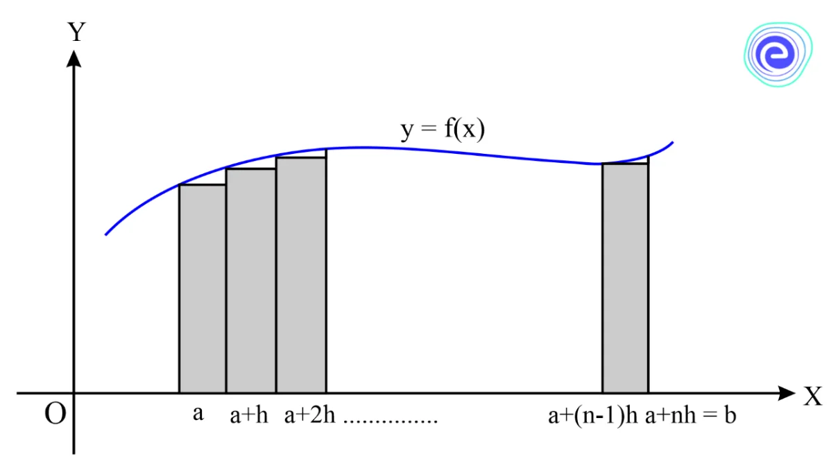
Let \(f\left( x \right)\) be a continuous real-valued function defined on the closed interval \(\left[ {a,b} \right]\), which is divided into \(n\) parts as shown below.

The points of division on the \(x-\) axis are \(a,a + h,a + 2h, \ldots a + (n – 1)h,a + nh\), where \(\frac{{b – a}}{n} = h\).

Left-End Estimation

Let \({L_n}\) denote the area of \(n\) rectangles.

Then, \(L_{n}=h f(a)+h f(a+h)+h f(a+2 h)+\ldots+h f(a+(n-1) h)\)

Clearly, \({L_n}\) represents an area very close to the area of the region bounded by curve \(y = f\left( x \right)\), \(x-\) axis and the ordinates \(x=a, x=b\).

Hence \(\int_a^b f (x)dx = \mathop {\lim }\limits_{n \to \infty } {L_n}\)
\(\int_a^b f (x)dx = \mathop {\lim }\limits_{n \to \infty } h[f(a) + f(a + h) + f(a + 2h) +  \ldots  + f(a + (n – 1)h)]\)
\( = \mathop {\lim }\limits_{n \to \infty } \sum\limits_{r = 0}^{n – 1} h f(a + rh),{\text{where }}nh = b – a\)
\( = \mathop {\lim }\limits_{n \to \infty } \sum\limits_{r = 0}^{n – 1} {\left( {\frac{{b – a}}{n}} \right)} f\left( {a + \left( {\frac{{b – a}}{n}} \right)r} \right)\)

If for a function \(f\left( x \right)\) the limit exists, we say the function is integrable on the interval \(\left[ {a,b} \right]\)

It can be shown that, when \(f\left( x \right)\) is a continuous function, the above limit always exists.

Hence, if a function \(f\left( x \right)\) is continuous on an interval \(\left[ {a,b} \right]\), then it is integrable on that interval.

Right-End Estimation

Considering the sum of areas of rectangles using the heights at the right-end points of the subintervals, we have

\({R_n} = hf(a + h) + hf(a + 2h) +  \ldots  + hf(a + nh)\)
\(\int_a^b f (x)dx = \mathop {\lim }\limits_{n \to \infty } \sum\limits_{r = 1}^n {\left( {\frac{{b – a}}{n}} \right)} f\left( {a + \left( {\frac{{b – a}}{n}} \right)r} \right)\)

It follows from theorem that for a continuous function \(f\),

\(\mathop {\lim }\limits_{n \to \infty } {R_n} = \mathop {\lim }\limits_{n \to \infty } {L_n} = \int_a^b f (x)dx\)

Hence, we can compute integral using either the left-end, or the right-end estimation.

Definite Integral as Generalised Limit of Sum

Let us consider a slightly different type of sum which is not necessarily either an upper sum or a lower sum or sum of areas of lower and upper rectangles, but which lies between them.

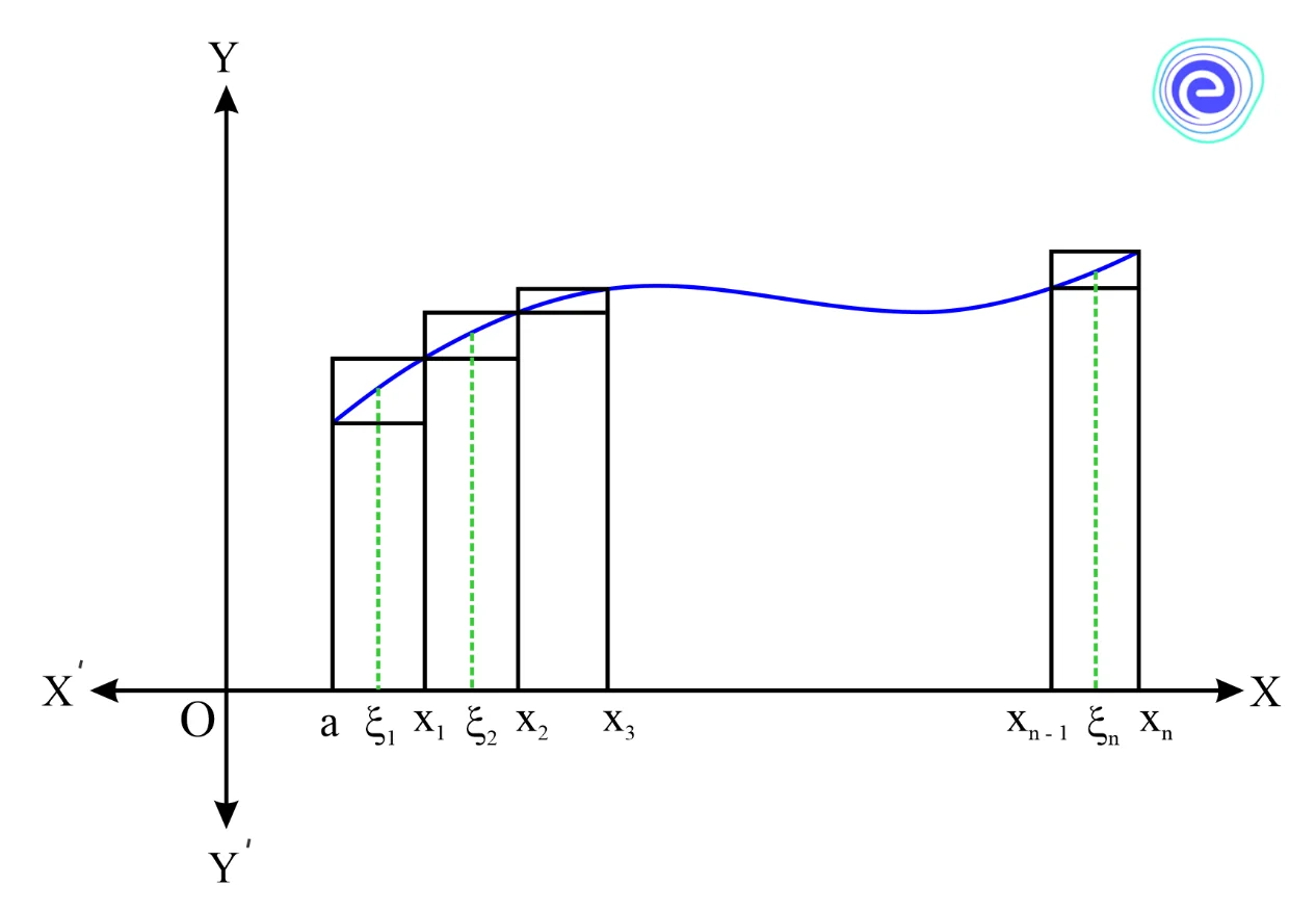
Given a partition \(P\) of an interval \(a \leqslant x \leqslant b\). We choose an arbitrary point \({\xi _r}\) (the symbol \(\xi \) is read as xi) in each sub-interval \(\left[ {{X_{r – 1}},{X_r}} \right],r = 1,2,3, \ldots ,n\).
If \(f\left( x \right)\) is bounded on \(\left[ {a,b} \right]\), then the sum
\({S_n} = \sum\limits_{r = 1}^n f \left( {{\xi _r}} \right)\Delta {X_r}\,\,\,\,\,\,\,……\left( 1 \right)\) will be called an integral sum or a Reimann sum, or approximating sum equal to the sum of the area of the rectangles.

Let us now make all \(\Delta {x_r} \to 0\) as \(\left\| P \right\|\, \to 0\,\) or \(n \to \infty \). If in doing so \({S_n}\) tends to definite limit \(S\), the area (in case of \(f\) is non-negative)
Hence \(S = \mathop {\lim }\limits_{||P|| \to 0} \sum\limits_{r = 1}^n f \left( {{\xi _r}} \right)\Delta {X_r}\,…….\left( 2 \right)\)

If the above limit exists and is finite, then we say that \(f\) is integrable on \(\left[ {a,b} \right]\), and this limit is called the definite integral of the function \(f\) on a closed interval \(\left[ {a,b} \right]\). It is denoted by \(\int_a^b f (x)dx\).
\(\therefore \,\,\,\mathop {\lim }\limits_{\left\| P \right\|\, \to 0} \sum\limits_{r = 1}^n f \left( {{\xi _r}} \right)\Delta {X_r} = \int_a^b f (x)dx\)

Note: In the symbol \(\int_a^b f (x)dx\), \(x\) is called the variable of integration, \(a\) is the lower limit, \(b\) is the upper limit and \(\left[ {a,b} \right]\) is called the range of the variable of integration \(x\).

Integral as a Function of Parameter

Let \(f:[a,b] \times [c,d] \to R\) if for each fixed \(t \in \left[ {c,d} \right]\) the function \(f\left( x,t \right)\) is integrable over \(\left[ {a,b} \right]\) on the \(x\) variable, we define the following function \(F:[a,b] \to R\) as
\(F(t) = \int_a^b f (x,t)dx\)
We call \(F\left( t \right)\) an integral depending on a parameter.

Theorem 1: If \(f\) continuous on \(\left[ {a,b} \right] \times \left[ {c,d} \right] \Rightarrow F\) is continuous on \(\left[ {c,d} \right]\).

Theorem 2: If \(f\) and \({f_t} = \frac{{\partial f}}{{\partial t}}\) continuous on \(\left[ {a,b} \right] \times \left[ {c,d} \right] \Rightarrow F\) is differentiable on \(\left[ {c,d} \right]\) and \(F'(t) = \int_a^b {{f_t}} (x,t)dx\)

Note: We can interchange the processes of integration and differentiation.

Theorem 3: (Leibniz’s Theorem)

Let \(f\) and \({f_t} = \frac{{\partial f}}{{\partial t}}\) be continuous functions on \(\left[ {a,b} \right] \times \left[ {c,d} \right]\) and \(\alpha ,\beta \) differentiable functions on \(\left[ {c,d} \right]\) with image on \(\left[ {a,b} \right]\), that is \(\alpha (t),\beta (t):[c,d] \to [a,b],x \in [\alpha (t),\beta (t)] \subset [a,b]\).
\(G(t) = \int_{a(t)}^{\beta (t)} f (x,t)dx\)
then \(G\) is differentiable on \(\left[ {c,d} \right]\)
\(\therefore {G^\prime }(t) = f(\beta (t),t) \cdot {\beta ^\prime }(t) – f(\alpha (t),t) \cdot {\alpha ^\prime }(t) + \int_{\alpha (t)}^{\beta (t)} {{f_t}} (x,t)dx\)

Integral as Infinite Sum

From the definition of definite integral, we have

1. \(\int_a^b f (x)dx = \mathop {\lim }\limits_{n \to \infty } \sum\limits_{r = 0}^{n – 1} {\left( {\frac{{b – a}}{n}} \right)} f\left( {a + \left( {\frac{{b – a}}{n}} \right)r} \right)\)
2. \(\int_a^b f (x)dx = \mathop {\lim }\limits_{n \to \infty } \sum\limits_{r = 1}^{n} {\left( {\frac{{b – a}}{n}} \right)} f\left( {a + \left( {\frac{{b – a}}{n}} \right)r} \right)\)
3. \(\mathop {\lim }\limits_{n \to \infty } \sum\limits_{r = 0}^{n – 1} {\left( {\frac{1}{n}} \right)} f\left( {\frac{r}{n}} \right) = \int_0^1 f (x)dx\)
4. \(\mathop {\lim }\limits_{n \to \infty } \frac{1}{n}\sum\limits_{r = \phi (x)}^{\psi (x)} f \left( {\frac{r}{n}} \right) = \int_a^b f (x)dx\), where
   (i) \(\sum {} \) is replaced by \(\int {} \)sign
   (ii) \(\frac{r}{n}\) is replaced by \(x\),
   (iii) \(\frac{1}{n}\) is replaced by \(dx\),
   (iv) To obtain the limits of integration, we use \(a = \mathop {\lim }\limits_{n \to \infty } \frac{{\phi (x)}}{n}\) and \(a = \mathop {\lim }\limits_{n \to \ } \frac{{\psi (x)}}{n}\)

Note: We have to see the following things before we can express the limit of its sum as a definite integral.

1. Each term of the series must be multiplied by \(\frac{1}{n}\) which tends to \(0\) when \(n \to \infty \).
2. All the terms should be some function of \(\frac{r}{n}\) which varies from term to term in A.P. with a common difference \(\frac{1}{n}\).

Solved Examples of Integral as Limit of Sum

Below are a few solved examples that can help in getting a better idea.

Q.1. Show that \(\int_0^1 {{x^2}} dx = \frac{1}{3}\).
Sol: Let \(P \to \left\{ {0,\frac{1}{n},\frac{2}{n},\frac{3}{n}, \ldots ,\frac{r}{n},\frac{n}{n}} \right\}\) be the points of partition \(P\) of \(\left[ {0,1} \right]\).
Here, \(f\left( x \right) = {x^2}\) is an increasing function in \(\left[ {0,1} \right]\).
Therefore, \(f\left( x \right) = {x^2}\) is increasing in \(\left[ {\frac{{r – 1}}{n},\frac{r}{n}} \right]\) and \({\delta _r} = \frac{1}{n}\)
\(\therefore {m_r} = f\left( {\frac{{r – 1}}{n}} \right) = \frac{{{{(r – 1)}^2}}}{{{n^2}}},{M_r} = f\left( {\frac{r}{n}} \right) = \frac{{{r^2}}}{{{n^2}}}\)
\(L(P,f) = \sum\limits_{r = 1}^{n – 1} {{m_r}} {\delta _r} = \sum\limits_{r = 1}^{n – 1} {\frac{{{{(r – 1)}^2}}}{{{n^2}}}}  = \frac{1}{{{n^3}}} \times \frac{{n(n – 1)(2n – 1)}}{6}\)
\(U(P,f) = \sum\limits_{r = 1}^n {{M_r}} {\delta _r} = \sum\limits_{r = 1}^n {\frac{{{r^2}}}{{{n^2}}}}  = \frac{1}{{{n^3}}} \times \frac{{n(n + 1)(2n + 1)}}{6}\)
As \(\left\| P \right\|\, \to 0\,i.e.,n \to \infty ,L(P,f) = U(P,f) \to \frac{1}{3}\)
Hence \(\int_0^1 {{x^2}} dx = \frac{1}{3}\).

Q.2. Calculate \(I = \int_0^2 {\left( {1+ {x^2}} \right)} dx\) as the limit of sums.
Sol: By definition, we have
\(\int_a^b f (x)dx = \mathop {\lim }\limits_{n \to \infty } h[f(a) + f(a + h) + f(a + 2h) +  \ldots  + f(a + (n – 1)h)]\)
Let \(f(x) = {x^2} + 1,a = 0,b = 2\) and \(nh = b – a = 2 – 0 = 2\)
\(\therefore \int_0^2 {\left( {1 + {x^2}} \right)} dx = \mathop {\lim }\limits_{h \to 0} h\left[ {1 + \left\{ {{h^2} + 1} \right\} + \left\{ {{{(2h)}^2} + 1} \right\} +  \ldots  + \left\{ {{{((n – 1)h)}^2} + 1} \right\}} \right]\)
\( = \mathop {\lim }\limits_{h \to 0} h\left[ {(1 + 1 + 1 +  \ldots  + 1) + \left\{ {{h^2} + {{(2h)}^2} +  \ldots  + {{((n – 1)h)}^2}} \right\}} \right]\)
\( = \mathop {\lim }\limits_{h \to 0} h\left[ {n + {h^2}\left\{ {{1^2} + {2^2} + {3^2} +  \ldots  + {{(n – 1)}^2}} \right\}} \right]\)
\( = \mathop {\lim }\limits_{h \to 0} h\left[ {n + {h^2} \cdot \frac{{(n – 1)n(2n – 1)}}{6}} \right]\)
\( = \mathop {\lim }\limits_{h \to 0} \left[ {nh + \frac{{(nh – h)nh(2nh – h)}}{6}} \right]\)
\( = \mathop {\lim }\limits_{h \to 0} \left[ {2 + \frac{{(2 – h)2((2 \cdot 2) – h)}}{6}} \right]\)
\( = 2 + \frac{{2 \cdot 2 \cdot 4}}{6}\)
\( = 2 + \frac{8}{3}\)
\( = \frac{{14}}{3}\)

Q.3. If \(f(x) = \int_0^x {(t + 1)} \left( {{e^t} – 1} \right)(t – 2)(t + 4)dt\), then find the points of local minima of \(f(x)\).
Sol: Using \({f^\prime }(x) = f(\beta (t),t) \cdot {\beta ^\prime }(t) – f(\alpha (t),t) \cdot {\alpha ^\prime }(t) + \int_{\alpha (t)}^{\beta (t)} {{f_t}} (x,t)dx\)
where \(\beta (t) = {x_1}\alpha (t) = 0\) and \({f_t} = \frac{{\partial f}}{{\partial t’}}\) we get
\({f^\prime }(x) = (x + 1)\left( {{e^x} – 1} \right)(x – 2)(x + 4)\)
The sign scheme for \({f^\prime }(x)\) is shown below.

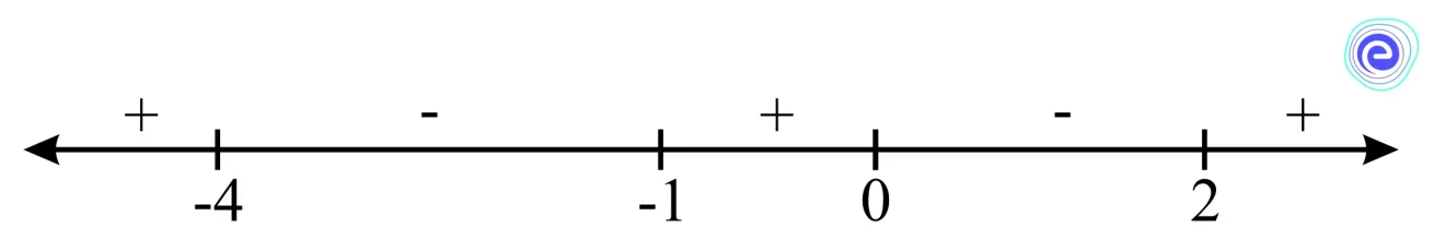
Clearly, \(x=-1\) and \(x=2\) are the points of local minima.

Q.4. Evaluate \(\mathop {\lim }\limits_{n \to \infty } \sum\limits_{i = 1}^n {\frac{2}{n}} \left[ {{{\left( {1 + \frac{{2i}}{n}} \right)}^2} + 1} \right]\)
Sol: \(\mathop {\lim }\limits_{n \to \infty } \sum\limits_{i = 1}^n {\frac{2}{n}} \left[ {{{\left( {1 + \frac{{2i}}{n}} \right)}^2} + 1} \right] = 2\int_0^1 {\left( {{{(1 + 2x)}^2} + 1} \right)} dx\)
\( = 2\left[ {\frac{{{{(1 + 2x)}^3}}}{{2 \cdot 3}} + x} \right]_0^1 = 2\left[ {\left( {\frac{{27}}{6} + 1} \right) – \frac{1}{6}} \right]\)
\( = 2\left[ {\frac{{27}}{6} + \frac{5}{6}} \right] = \frac{{32}}{3}\)

Q.5. If \(\int_1^{\sin x} {{t^2}} f(t)dt = 1 – \sin x\), where \(x \in \left( {0,\frac{\pi }{2}} \right)\), then find the value of \(f\left( {\frac{1}{{\sqrt 3 }}} \right)\)
Sol: We have \(\int_1^{\sin x} {{t^2}} f(t)dt = 1 – \sin x\)
Differentiating both sides, we get
\( – {\sin ^2}xf(\sin x)\cos x =  – \cos x\)
\( \Rightarrow f(\sin x) = {\operatorname{cosec} ^2}x = \frac{1}{{{{\sin }^2}x}},x \in \left( {0,\frac{\pi }{2}} \right)\)
\( \Rightarrow f(z) = \frac{1}{{{z^2}}},z \in (0,1)\)
\(\therefore f\left( {\frac{1}{{\sqrt 3 }}} \right) = 3\)

Summary

There are two types of integrals: Indefinite and definite integrals. Definite integrals can be solved as the limit of a sum. Alternatively, if there exists an antiderivative \(F\) for the interval \(\left[ {a,b} \right]\), the definite integral of the function is the difference of the values at points \(a\) and \(b\). For definite integrals, using the Reimann sum, we get \(\int_a^b f (x)dx = \mathop {\lim }\limits_{n \to \infty } \sum\limits_{r = 1}^n {{m_r}} {\delta _r} = \mathop {\lim }\limits_{n \to \infty } \sum\limits_{r = 1}^n {{M_r}} {\delta _r}\), where \(U(P,f) = \sum\limits_{r = 1}^n {{M_r}} {\delta _r}\) and \(L(P,f) = \sum\limits_{r = 1}^n {{m_r}} {\delta _r}\). The numbers \(L(P,f),\,U(P,f)\) are respectively the lower and upper Reimann integrals of \(f\). Integral as a limit of the sum is \(\int_a^b f (x)dx = \mathop {\lim }\limits_{n \to \infty } \sum\limits_{r = 0}^{n – 1} {\left( {\frac{{b – a}}{n}} \right)} f\left( {a + \left( {\frac{{b – a}}{n}} \right)r} \right) = \mathop {\lim }\limits_{n \to \infty } \sum\limits_{r = 1}^n {\left( {\frac{{b – a}}{n}} \right)} f\left( {a + \left( {\frac{{b – a}}{n}} \right)r} \right)\). Lastly, Leibniz’s theorem states that if \(G(t) = \int_{\alpha (t)}^{\beta (t)} f (x,t)dx\) then \(G\) is differentiable on \(\left[ {c,d} \right]\) and \({G^\prime }(t) = f(\beta (t),t) \cdot {\beta ^\prime }(t) – f(\alpha (t),t) \cdot {\alpha ^\prime }(t) + \int_{\alpha (t)}^{\beta (t)} {{f_t}} (x,t)dx\).

Frequently Asked Questions (FAQs)

The frequently asked questions on Integral as Limit of Sum are given below:

Q.1. How do you rewrite an integral as a limit?
Ans: Definite integral as a limit of the sum is calculated as
\(\int_a^b f (x)dx = \mathop {\lim }\limits_{n \to \infty } \sum\limits_{r = 0}^{n – 1} {\left( {\frac{{b – a}}{n}} \right)} f\left( {a + \left( {\frac{{b – a}}{n}} \right)r} \right) = \mathop {\lim }\limits_{n \to \infty } \sum\limits_{r = 1}^n {\left( {\frac{{b – a}}{n}} \right)} f\left( {a + \left( {\frac{{b – a}}{n}} \right)r} \right)\)

Q.2. What is the limit of the sum?
Ans: If \(f\left( x \right)\) is a continuous real-valued function defined on the closed interval \(\left[ {a,b} \right]\) divided into \(n\) parts.
The points of division on the \(x-\) axis are \(a,a + h,a + 2h, \ldots a + (n – 1)h,a + nh\), where \(\frac{{b – a}}{n} = h\). Then
\(\int_a^b f (x)dx = \mathop {\lim }\limits_{n \to \infty } h[f(a) + f(a + h) + f(a + 2h) +  \ldots  + f(a + (n – 1)h)]\)

Q.3. What is the definite integral limit of Riemann sums?
Ans: The sum \(U(P,f) = \sum\limits_{r = 1}^n {{M_r}} {\delta _r}\) and \(L(P,f) = \sum\limits_{r = 1}^n {{m_r}} {\delta _r}\), will respectively be called the upper-integral sum and the lower-integral sum of \(f\) over the partition \(P\) of \(\left[ {a,b} \right]\).
If \(f:\left[ {a,b} \right] \to R\) is a bounded function. Then \(f\) is said to be integral on \(\left[ {a,b} \right]\). If \(L\left( {P,f} \right) = U\left( {P,f} \right)\) (As \(n \to \infty \) or \(\left\| P \right\| \to 0\)). In this case, the common value \(U\left( {P,f} \right) = L\left( {P,f} \right)\) is called the Reimann integral of \(f\) on \(\left[ {a,b} \right]\). It is denoted by \(\int_a^b f (x)dx\).
\(\therefore \int_a^b f (x)dx = \mathop {\lim }\limits_{n \to \infty } \sum\limits_{r = 1}^n {{m_r}} {\delta _r} = \mathop {\lim }\limits_{n \to \infty } \sum\limits_{r = 1}^n {{M_r}} {\delta _r}\)

Q.4. What is the integral sum rule?
Ans: The integral sum rules are:
1. \(\int_a^b f (x)dx = \mathop {\lim }\limits_{n \to \infty } \sum\limits_{r = 0}^{n – 1} {\left( {\frac{{b – a}}{n}} \right)} f\left( {a + \left( {\frac{{b – a}}{n}} \right)r} \right)\)
2. \(\int_a^b f (x)dx = \mathop {\lim }\limits_{n \to \infty } \sum\limits_{r = 1}^{n} {\left( {\frac{{b – a}}{n}} \right)} f\left( {a + \left( {\frac{{b – a}}{n}} \right)r} \right)\)
3. \(\mathop {\lim }\limits_{n \to \infty } \sum\limits_{r = 0}^{n – 1} {\left( {\frac{1}{n}} \right)} f\left( {\frac{r}{n}} \right) = \int_0^1 f (x)dx\)
4. \(\mathop {\lim }\limits_{n \to \infty } \frac{1}{n}\sum\limits_{r = \phi (x)}^{\psi (x)} f \left( {\frac{r}{n}} \right) = \int_a^b f (x)dx\), where
(i) \(\sum {} \) is replaced by \(\int {} \)sign
(ii) \(\frac{r}{n}\) is replaced by \(x\),
(iii) \(\frac{1}{n}\) is replaced by \(dx\),
(iv) To obtain the limits of integration, we use \(a = \mathop {\lim }\limits_{n \to \infty } \frac{{\phi (x)}}{n}\) and \(b = \mathop {\lim }\limits_{n \to \ } \frac{{\psi (x)}}{n}\)

Q.5. What is the integral of \(0\)?
Ans: Since \(0\) is a constant and we know that
\(\int {c\,dx\, = cx} \), where \(c\) is a constant
Therefore, \(\int {0\,dx\, = 0\, \cdot \,x = 0} \)
Hence, the integral of \(0\) is \(0\)

We hope this information about the Integral as Limit of Sum has been helpful. If you have any doubts, comment in the section below, and we will get back to you soon.