Limits of Polynomials and Rational Functions: Limits are calculus’s fundamental concept. They are required in both differential and integral calculus. The range of variables over which the operation is performed is the limits of the operation. This means that every calculation of calculus involves limits in one way or the other. The simplest and the most common application of limits is the speedometer in your car. We know that it measures the instantaneous velocity of the vehicle, but, mathematically, it is described as the maximum change in distance in the given time as it gets shorter.

In this article, let us learn how to apply limits for polynomials and rational functions along with some solved examples.

What are Limits?

A limit is a value that the output of a function approaches as the input of the function approaches a given value. It is a mathematical idea that is based on closeness, and it is widely used to assign values to functions even at points where no values are defined.

For example, \(f(x)=\frac{1}{x-1}\) is not defined for \(x = 1\), as dividing by zero is mathematically undefined.

Limit of \(f(x)\) at \(x_{0}\) is defined as,

\(\mathop {\lim }\limits_{x \to {x_0}} f(x)\)

This means that there is a \(g(x)\) such that \(g(x)=f(x)\) in an interval around \(x_{0}\), except at \(x_{0}\) itself. 

What are the Limits of Polynomials?

A function defined by an expression with at least one algebraic term is called a polynomial function. If \(f(x)\) is a polynomial function of degree \(n\), then, 

\(f(x)=a_{0}+a_{1} x+a_{2} x^{2}+\ldots+a_{n} x^{n}\)

where \(a_{i} \mathrm{~s}\) are real numbers such that \(a_{n} \neq 0\), for any real number \(n\).

As we know

\(\mathop {\lim }\limits_{x \rightarrow a} x=a\)

\(\mathop {\lim }\limits_{x \to a} {x^2} = \mathop {\lim }\limits_{x \to a} (x \cdot x)\)

\( = \mathop {\lim }\limits_{x \to a} x \cdot \mathop {\lim }\limits_{x \to a} x\)

\(=a.a\)

\(\therefore \mathop {\lim }\limits_{x \rightarrow a} x^{2}=a^{2}\)

Similarly, we can write the limit of \(x^{n}\) as,

\(\mathop {\lim }\limits_{x \rightarrow a} x^{n}=a^{n}\)

From these, we can write the limit of the polynomial function,

\(f(x)=a_{0}+a_{1} x+a_{2} x^{2}+\cdots+a_{n} x^{n}\)

by considering each term i.e., \(a_{0}, a_{1} x, a_{2} x^{2}, \ldots a_{n} x^{n}\) as functions.

\(\mathop {\lim }\limits_{x \to a} f(x) = \mathop {\lim }\limits_{x \to a} \left[ {{a_0} + {a_1}x + {a_2}{x^2} +  \cdots  + {a_n}{x^n}} \right]\)

By distributive property, splitting the limit for each term,

\(\mathop {\lim }\limits_{x \to a} f(x) = \mathop {\lim }\limits_{x \to a} {a_0} + \mathop {\lim }\limits_{x \to a} {a_1}x + \mathop {\lim }\limits_{x \to a} {a_2}{x^2} +  \cdots  + \mathop {\lim }\limits_{x \to a} {a_n}{x^n}\)

Now, take the constants out of each limit,

\(\mathop {\lim }\limits_{x \to a} f(x) = {a_0} + {a_1}\mathop {\lim }\limits_{x \to a} x + {a_2}\mathop {\lim }\limits_{x \to a} {x^2} +  \cdots  + {a_n}\mathop {\lim }\limits_{x \to a} {x^n}\)

Therefore,

\(\mathop {\lim }\limits_{x \to a} f(x) = {a_0} + {a_1}a + {a_2}{a^2} +  \cdots  + {a_n}{a^n} = f(a)\)

\(\Rightarrow \mathop {\lim }\limits_{x \to a} f(x) = f(a)\)

Limits of Rational Functions

A function that can be written as the ratio of two polynomial functions such that the denominator of the function is not zero is called a rational function. If \(f(x)\) is called a rational function, then,

\(f(x)=\frac{g(x)}{h(x)}\)

Where \(g(x)\) and \(h(x)\) are polynomial functions, such that \(h(x) \neq 0\)

The application of limit for \(f(x)\) as \(x\) tends to \(c\) is given as,

\(\mathop {\lim }\limits_{x \to c} f(x) = \mathop {\lim }\limits_{x \to c} \frac{{g(x)}}{{h(x)}} = \frac{{\mathop {\lim }\limits_{x \to c} g(x)}}{{\mathop {\lim }\limits_{x \to c} h(x)}} = \frac{{g(c)}}{{h(c)}}\)

If \(h(c)=0\), then we consider two cases to define the limits of the rational function.

Case 1: \(g(c) \neq 0\)

Since, \(g(c) \neq 0\) and \(h(c)=0\), the limit does not exist.

Case 2: \(g(c)=0\)

In this case, we need to write the functions \(g(x)\) and \(h(x)\) as,

\(g(x)=(x-c)^{k} g_{1}(x)\)

where \(k\) is the maximum of powers of \((x-c)\) in \(g(x)\),

\(h(x)=(x-c)^{l} h_{1}(x)\) as \(h(c)=0\)

Assume \(k>l\), then we have,

\(\mathop {\lim }\limits_{x \to c} f(x) = \mathop {\lim }\limits_{x \to c} \frac{{g(x)}}{{h(x)}}\)

\( = \frac{{\mathop {\lim }\limits_{x \to c} g(x)}}{{\mathop {\lim }\limits_{x \to c} h(x)}}\)

\(\therefore \mathop {\lim }\limits_{x \to c} f(x) = \frac{{\mathop {\lim }\limits_{x \to c} {{(x – c)}^k}{g_1}(x)}}{{\mathop {\lim }\limits_{x \to c} {{(x – c)}^l}{h_1}(x)}}\)

By applying the quotient rule of exponents, we get,

\(\frac{{\mathop {\lim }\limits_{x \to c} {{(x – c)}^k}{g_1}(x)}}{{\mathop {\lim }\limits_{x \to c} {{(x – c)}^l}{h_1}(x)}} = \frac{{\mathop {\lim }\limits_{x \to c} {{(x – c)}^{(k – l)}}{g_1}(x)}}{{\mathop {\lim }\limits_{z \to c} {h_1}(x)}}\)

\(= \frac{{0 \times {g_1}(c)}}{{{h_1}(c)}}\)

\(=0\)

However, when \(k<l\) the limit does not exist.

Thus, we need to evaluate the functions individually that are involved in the rational functions. At the prescribed points at first, if this is of the form \(\frac{0}{0}\). So in this case, we have to write the function in terms of factors such that we could cancel the common factors which are causing the limit to be of the form \(\frac{0}{0}\).

Limits of Polynomials at Infinity

Consider the functions \(f(x)=\frac{1}{x}\) and \(f(x)=\frac{1}{x^{2}}\)

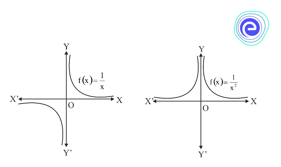
We observe from the graph that as \(x\) increases, the values of \(f(x)=\frac{1}{x}\) and \(f(x)=\frac{1}{x^{2}}\) decrease rapidly. When \(x\) is large \(\frac{1}{x}\) and \(\frac{1}{x^{2}}\) are very close to zero. In cases such as

\(\mathop {\lim }\limits_{x \rightarrow+\infty} \frac{1}{x}=0\) and \(\mathop {\lim }\limits_{x \rightarrow+\infty} \frac{1}{x^{2}}=0\)

We also observe from the graphs of these two functions that as \(x\) decreases and when \(x\) is a small negative number, the values of \(\frac{1}{x}\) and \(\frac{1}{x^{2}}\) approach to zero. So, we can write,

\(\mathop {\lim }\limits_{x \rightarrow-\infty} \frac{1}{x}=0\) and \(\mathop {\lim }\limits_{x \rightarrow-\infty} \frac{1}{x^{2}}=0\)

From the above discussion, we can write,

1. \(\mathop {\lim }\limits_{x \rightarrow \infty} c=c\)

2. \(\mathop {\lim }\limits_{x \rightarrow-\infty} c=c\)

3. \(\mathop {\lim }\limits_{x \rightarrow \infty} \frac{c}{x^{n}}=0, n>0\)

4. \(\mathop {\lim }\limits_{x \rightarrow-\infty} \frac{c}{x^{n}}=0, n \in N\)

We use these above results to evaluate polynomials at infinity.

Algorithm to Evaluate Limits at Infinity

This algorithm can be used to evaluate limits at Infinity.

Step 1: Write the given expression in the form of a rational function i.e. \(\frac{f(x)}{g(x)}\)

Step 2: If \(k\) is the highest power of \(x\) in numerator and denominator, then divide each term in numerator and denominator by \(x^{k}\).

Step 3: Use the standard results such as \(\mathop {\lim }\limits_{x \rightarrow \infty} \frac{c}{x^{n}}=0\) and \(\mathop {\lim }\limits_{x \rightarrow \infty} c=c\) where \(n>0\) and simplify.

Example:

Evaluate \(\mathop {\lim }\limits_{x \rightarrow \infty} \frac{a x^{2}+b x+c}{d x^{2}+e x+f}\)

Solution:

Notice that the highest power of \(x\) in both numerator and denominator is \(2\).

So, we divide each term in both numerator and denominator by \(x^{2}\).

\(\therefore \mathop {\lim }\limits_{x \to \infty } \frac{{a{x^2} + bx + c}}{{d{x^2} + ex + f}} = \mathop {\lim }\limits_{x \to \infty } \frac{{a + \frac{b}{x} + \frac{c}{{{x^2}}}}}{{d + \frac{e}{x} + \frac{f}{{{x^2}}}}}\)

\( = \frac{{a + 0 + 0}}{{d + 0 + 0}}\)

\(\therefore \mathop {\lim }\limits_{x \to \infty } \frac{{a{x^2} + bx + c}}{{d{x^2} + ex + f}} = \frac{a}{d}\)

Evaluating Limits of Polynomials

When we evaluate \(\mathop {\lim }\limits_{x \to a} f(x)\) we do one of the following:

• Find the limit value \(L\) (in simplified form), we write \(\mathop {\lim }\limits_{x \rightarrow a} f(x)=L\)
• Say that, the limit is infinity \((\infty)\) or negative infinity \((-\infty)\) we write \(\mathop {\lim }\limits_{x \to a} f(x) = \infty \) or \(\mathop {\lim }\limits_{x \rightarrow a} f(x)=-\infty\)

When the limit \(\infty\)is  or \(-\infty\), the limit is still non-existent. So \(\mathop {\lim }\limits_{x \rightarrow a} f(x)\) is called limit at a point, because \(x=a\) corresponds to a point on the real number line.  Sometimes this is related to a point on the graph of the function.

Algorithm

To evaluate the limit of a polynomial at \(x=a\), we can follow these steps.

Step 1: Use the properties of limits to break up the polynomial into individual terms.

Step 2: Find the limits of the individual terms.

Step 3: Add the limits together.

Step 4: Alternatively, evaluate the function for \(a\).

Evaluating Limits of Rational Functions

To evaluate the limit of rational functions, we can use the following methods.

Direct Substitution Method

Consider the limit, \(\mathop {\lim }\limits_{x \to a} \frac{{\varphi (x)}}{{\psi (x)}}\), if \(\frac{\varphi(a)}{\psi(a)}\) exists and a fixed real number at \(x=a\), then we say that, \(\mathop {\lim }\limits_{x \rightarrow a} \frac{\varphi(x)}{\psi(a)}=\frac{\varphi(a)}{\psi(a)}\). In other words, the direct substitution method at a point, to which the variable tends to, we obtain a fixed real number, then the number obtained is the limit of the function. In fact, if the point to which the variable tends to is a point in the domain of the function, then the value of the function at that point is its limit.

Factorization Method

Consider the limit \(\mathop {\lim }\limits_{x \rightarrow a} \frac{f(x)}{g(x)}\) . If by substituting \(x=a\) then \(\frac{f(x)}{g(x)}\) is reduces to \(\frac{0}{0}\), then \((x-a)\) is a factor of \(f(x)\) and \(g(x)\) both. We first factorize \(f(x)\) and \(g(x)\) then cancel out the common factor to evaluate the limit.

The following algorithm may be used to evaluate the limit by the factorization method.

Algorithm

Step 1: Obtain the problem I say, \(\mathop {\lim }\limits_{x \rightarrow a} \frac{f(x)}{g(x)}\), where \(\mathop {\lim }\limits_{x \rightarrow a} f(x)=0\) and \(\mathop {\lim }\limits_{x \rightarrow a} g(x)=0\)

Step 2: Factorize \(f(x)\) and \(g(x)\)

Step 3: Cancel out the common factor(s) of \(f(x)\) and \(g(x)\)

Step 4: Use the direct substitution method to find the limit.

Rationalization Method

This method is particularly used to find the limits of a rational function, when:

• The numerator or denominator or both involve expressions consisting of square roots.
• Substituting the value of \(x\) the rational expression takes the form \(\frac{0}{0}, \frac{\infty}{\infty}\) etc.

In this method, we multiply the rational function by a form of \(1\) such that it eliminates radical symbols and imaginary numbers in the denominator. This avoids the chance of getting a zero in the denominator when the limits are substituted.

Solved Examples

Q.1. Compute \(\mathop {\lim }\limits_{x \rightarrow 2}\left[x^{3}-x^{2}+2\right]\)
Ans: Given that, we have, \(\mathop {\lim }\limits_{x \rightarrow 2}\left[x^{3}-x^{2}+2\right]\)

We know that, \(\mathop {\lim }\limits_{x \rightarrow a} f(x)=f(a)\)

Therefore, \(\mathop {\lim }\limits_{x \rightarrow 2}\left[x^{3}-x^{2}+2\right]=(2)^{3}-(2)^{2}+2\)

\(=8-4+2=6\)

\(\therefore \mathop {\lim }\limits_{x \rightarrow 2}\left[x^{3}-x^{2}+2\right]=6\)

Q.2. Compute \(\mathop {\lim }\limits_{x \rightarrow 2} \frac{x^{2}-4}{x+3}\)
Ans: Using the direct substitution method, we have

\(\mathop {\lim }\limits_{x \rightarrow 2} \frac{x^{2}-4}{x+3}\)

\(=\frac{4-4}{2+3}\)

\(=\frac{0}{5}\)

Hence, \(\mathop {\lim }\limits_{x \rightarrow 2} \frac{x^{2}-4}{x+3}=0\)

Q.3. Evalute \(\mathop {\lim }\limits_{x \rightarrow 2} \frac{x^{2}-5 x+6}{x^{2}-4}\)
Ans: When \(x=2\) the expression \(\frac{x^{2}-5 x+6}{x^{2}-4}\) is assumes the indeterminate form \(\frac{0}{0}\). Therefore \((x-2)\) is a common factor in numerator and denominator. Factorising the numerator and denominator, we obtain \(\mathop {\lim }\limits_{x \rightarrow 2} \frac{x^{2}-5 x+6}{x^{2}-4}\)

\(=\mathop {\lim }\limits_{x \rightarrow 2} \frac{(x-2)(x-3)}{(x+2)(x-2)}\)

\(=\mathop {\lim }\limits_{x \rightarrow 2} \frac{x-3}{x+2}\)

\(=\frac{2-3}{2+2}\)

Hence, \(\mathop {\lim }\limits_{x \rightarrow 2} \frac{x^{2}-5 x+6}{x^{2}-4}=-\frac{1}{4}\)

Q.4. Evaluate \(\mathop {\lim }\limits_{x \rightarrow 2} \frac{x^{3}-3 x^{2}+4}{x^{4}-8 x^{2}+16}\)
Ans: When \(x=2\) the expression \(\frac{x^{3}-3 x^{2}+4}{x^{4}-8 x^{2}+16}\) is assumes the indeterminate form \(\frac{0}{0} .\) Therefore \((x-2)\) is a common factor in numerator and denominator. Factorising the numerator and denominator, we obtain \(\mathop {\lim }\limits_{x \to 2} \frac{{{x^3} – 3{x^2} + 4}}{{{x^4} – 8{x^2} + 16}} = \mathop {\lim }\limits_{x \to 2} \frac{{(x – 2)\left( {{x^2} – x – 2} \right)}}{{{{\left( {{x^2} – 4} \right)}^2}}}\)

\(=\mathop {\lim }\limits_{x \rightarrow 2} \frac{(x-2)(x-2)(x+1)}{(x-2)^{2}(x+2)^{2}}\)

\(=\mathop {\lim }\limits_{x \rightarrow 2} \frac{x+1}{(x+2)^{2}}\)

\(=\frac{2+1}{(2+2)^{2}}\)

Hence, \(\mathop {\lim }\limits_{x \rightarrow 2} \frac{x^{3}-3 x^{2}+4}{x^{4}-8 x^{2}+16}=\frac{3}{16}\)

Q.5. Evaluate \(\mathop {\lim }\limits_{x \rightarrow 0} \frac{\sqrt{a^{2}+x^{2}}-\sqrt{a^{2}-x^{2}}}{x^{2}}\)
Ans: When \(x=0\), the expression \(\frac{\sqrt{a^{2}+x^{2}}-\sqrt{a^{2}-x^{2}}}{x^{2}}\) takes the form \(\frac{0}{0}\). Rationlising the numerator, we get \(\mathop {\lim }\limits_{x \to 0} \frac{{\sqrt {{a^2} + {x^2}}  – \sqrt {{a^2} – {x^2}} }}{{{x^2}}} = \mathop {\lim }\limits_{x \to 0} \frac{{\left( {\sqrt {{a^2} + {x^2}}  – \sqrt {{a^2} – {x^2}} } \right)\left( {\sqrt {{a^2} + {x^2}}  + \sqrt {{a^2} – {x^2}} } \right)}}{{\left( {\sqrt {{a^2} + {x^2}}  + \sqrt {{a^2} – {x^2}} } \right)}}\) [Form \(\frac{0}{0}\), so apply rationlisation method]

\(=\mathop {\lim }\limits_{x \rightarrow 0} \frac{a^{2}+x^{2}-a^{2}+x^{2}}{x^{2}\left(\sqrt{a^{2}+x^{2}}+\sqrt{a^{2}-x^{2}}\right)}\)

\(=\mathop {\lim }\limits_{x \rightarrow 0} \frac{2}{\left(\sqrt{a^{2}+x^{2}}+\sqrt{a^{2}-x^{2}}\right)}\)

\(=\frac{2}{\sqrt{a^{2}}+\sqrt{a^{2}}}\)

\(=\frac{2}{2 \sqrt{a^{2}}}\)

\(\therefore \mathop {\lim }\limits_{x \rightarrow 0} \frac{\sqrt{a^{2}+x^{2}}-\sqrt{a^{2}-x^{2}}}{x^{2}}=\frac{1}{a}\)

Q.6. Evaluate \(\mathop {\lim }\limits_{x \rightarrow \infty} \frac{5 x-6}{\sqrt{4 x^{2}+9}}\)
Ans: We have, \(\mathop {\lim }\limits_{x \rightarrow \infty} \frac{5 x-6}{\sqrt{4 x^{2}+9}}\)
Now, dividing numerator and denominator by \(x\), then we get: \(\mathop {\lim }\limits_{x \to \infty } \frac{{5x – 6}}{{\sqrt {4{x^2} + 9} }} = \mathop {\lim }\limits_{x \to \infty } \frac{{5 – \frac{6}{x}}}{{\sqrt {4 + \frac{9}{{{x^2}}}} }}\)
\(=\frac{5-0}{\sqrt{4+0}}\)
\(\therefore \mathop {\lim }\limits_{x \rightarrow \infty} \frac{5 x-6}{\sqrt{4 x^{2}+9}}=\frac{5}{2}\)

Summary

A limit is a value that the output of a function approaches as the input of the function approaches a given value. In this article, we learn to apply limits to polynomial functions, and rational functions. We studied how we find the value of the limits at a prescribed point by using different methods such as direct substitution method, factorisation method, rationalisation method and reduction to standard forms.

Frequently Asked Questions (FAQs)

Q.1. What is the limit of a polynomial function?
Ans:  A limit of a polynomial function is the sum of all the limits of its individual terms.

Q.2. Which technique is useful when finding the limit of a rational function?
Ans:
Step 1: Factor the numerator.
Step 2: Cancel any common factors with the numerator.
Step 3: Apply the limits.
Step 4: Simplify.

Q.3. How do you find the infinite limits of a rational function?
Ans: To evaluate the limits at infinity for a rational function, we divide the numerator and denominator by the highest power of \(x\) appearing in the denominator. This helps us determine which term dominates the behaviour of the function for large values of \(x\).

Q.4. How do you find the limit of a rational polynomial?
Ans: For the rational function \(f(x)=\frac{p(x)}{q(x)}\) and for any real \(a,\mathop {\lim }\limits_{x \to a} f(x) = \frac{{p(a)}}{{q(a)}}\) If \(q(a) \ne 0\)
If \(q(a)=0\), then the function may or may not have a limit.
For the rational function \(f(x)=\frac{p(x)}{q(x)}=\frac{a_{n} x^{n}+a_{n-1} x^{n-1}+\cdots+a_{2} x^{2}+a_{1} x+a_{0}}{b_{m} x^{m}+b_{m-1} x^{m-1}+\cdots+b_{2} x^{2}+b_{1} x+b_{0}}\)
\(\mathop {\lim }\limits_{x \to  \pm \infty } f(x) = \left( {\frac{{{a_n}}}{{{b_m}}}} \right) \cdot \mathop {\lim }\limits_{x \to \infty } {x^{n – m}} = \left\{ {\begin{array}{*{20}{l}} { + \infty \;{\rm{ or }}\; – \infty }&{{\rm{ if }}\; n > m}\\{\frac{{{a_n}}}{{{b_m}}}}&{{\rm{ if }}\; n = m}\\0&{{\rm{ if }}\; n < m}\end{array}} \right.\)

Q.5. Why are there no restrictions for polynomial functions?
Ans: Polynomials may have any number of power functions added together. Hence, there is no specific count or limit to the number of parameters used here.

Learn about Functions here

Hope this detailed article on the Limits of Polynomials and Rational Functions helps you in your preparation. In case of any query, reach out to us in the comment section and we will get back to you at the earliest.