Line of Regression: Applying a linear equation to observed data, linear regression attempts to demonstrate the relationship between two variables. One variable is independent, while the other is dependent. For example, the weight of a person is proportional to their height. We can say that a linear relationship exists between the person’s height and weight. The weight of a person increases in proportion to their height.

Regression coefficients are estimates of unknown parameters that describe the relationship between a predictor variable and its corresponding response. In this article, let us learn about the line of regression, including its definition, equation and coefficients.

Line of Regression: What is a Regression Line?

A line that describes how a set of data behaves is called a regression line. In other words, it provides the best trend from the available data.

One variable is not required to be dependent on another, or that one causes changes in the other, but there must also be some critical relationship between the two variables. In such cases, a scatter plot indicates the strength of the relationship between the variables.

The scatter plots do not show any increasing or decreasing pattern if there is no relationship or linking between the variables. In such cases, the linear regression is ineffective with the given data.

Equation of Line of Regression

The correlation coefficient defines the strength of a relationship between two variables. This coefficient’s value ranges from -1 to +1. This coefficient represents the strength of the observed data’s association with two variables.

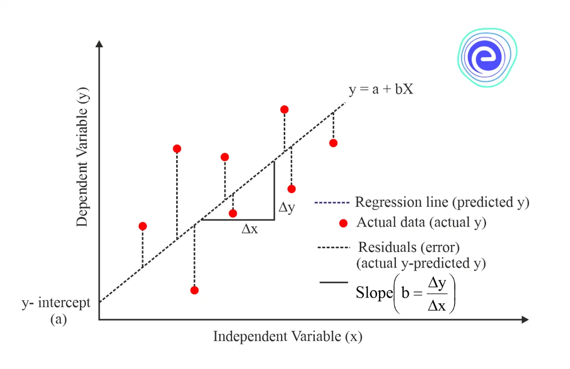
A linear regression line equation is written as y = a + bx, where x is the independent variable and is plotted along the x-axis.

The dependent variable, y, is plotted along the y-axis. The line’s slope is b, and the y-intercept is a.

Linear Regression

Linear regression depicts the relationship between two variables in a linear fashion. The linear regression equation is similar to the slope formula. It is calculated as \(y = a + bx\).

Now, let us determine the value of the slope of the line, \(b\), and the \(y\)-intercept, \(a\).

\(a = \frac{{\left( {\sum y } \right)\left( {\sum {{x^2}} } \right) – \left( {\sum x } \right)\left( {\sum x y} \right)}}{{n\left( {\sum {{x^2}} } \right) – {{\left( {\sum x } \right)}^2}}}\) and \({\rm{ }}b = \frac{{\left( {\sum x y} \right) – \left( {\sum x } \right)\left( {\sum y } \right)}}{{n\left( {\sum {{x^2}} } \right) – {{\left( {\sum x } \right)}^2}}}\)

Simple Linear Regression

Simple linear regression is the primary cause of a single scalar predictor variable x and a single scalar response variable y. This regression equation is represented as \(y = a + bx\)

A multiple linear regression, also known as multivariable linear regression, is the extension to multiple and vector-valued predictor variables. 

Almost all real-world regression patterns contain multiple predictors, and explanations of linear regression are frequently expressed in terms of the multiple regression form. However, in these cases, the dependent variable y is still a scalar.

Regression Analysis

Regression coefficients are estimates of unknown parameters that describe the relationship between a predictor variable and its corresponding response. We can say that regression coefficients are used to forecast the value of an unknown variable based on the value of a known variable.

Linear regression determines the straight-line equation that quantifies how a unit change in an independent variable causes a change in the dependent variable. This is referred to as regression analysis.

Correlation Coefficients

Correlation coefficient is a statistical concept that assists in establishing a relationship between predicted and actual values obtained in an experiment. The calculated correlation coefficient value explains the closeness of the predicted and actual values.

The value of the correlation coefficients lies between \(-1\) and \(+1\). If the correlation coefficient value is positive, the two variables have a similar and identical relationship.

Otherwise, it denotes the dissimilarity of the two variables. It is expressed as a number known as the correlation coefficient. Correlations are classified into three types:

Positive Correlation	The value of one variable increases linearly as the value of the other variable increases. This indicates that both variables have a similar relationship. In this case, the correlation coefficient would be positive, or \(1\).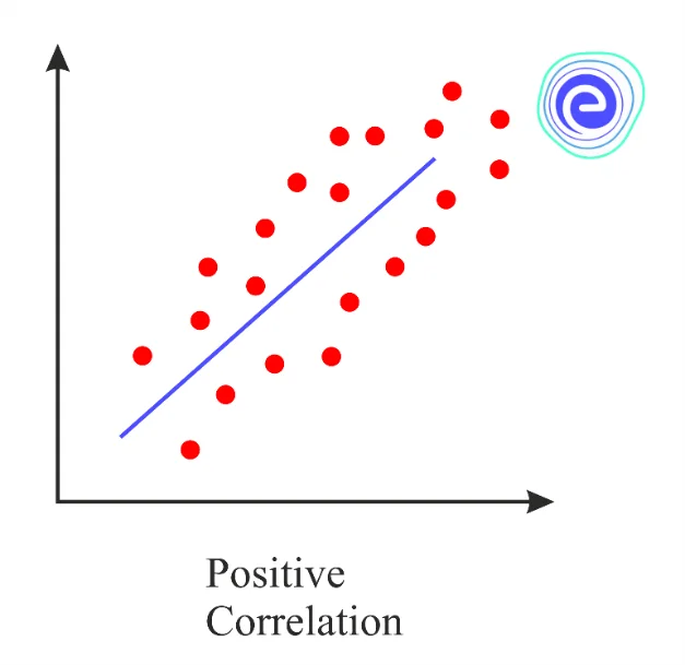
Negative Correlation	When the value of one variable fall while the values of the other variable fall, it is said to be negatively correlated. The correlation coefficient would be negative in that case.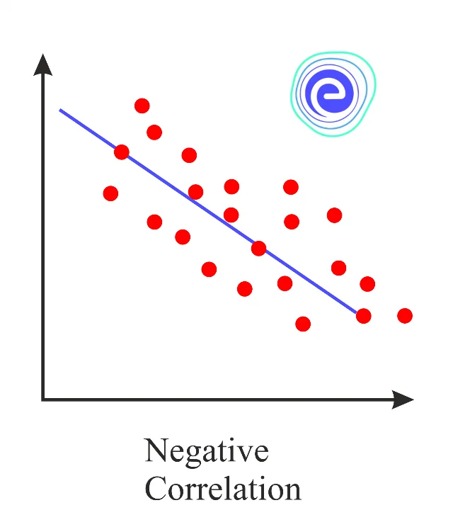
Zero Correlation	Another situation occurs when there is no specific relationship between two variables.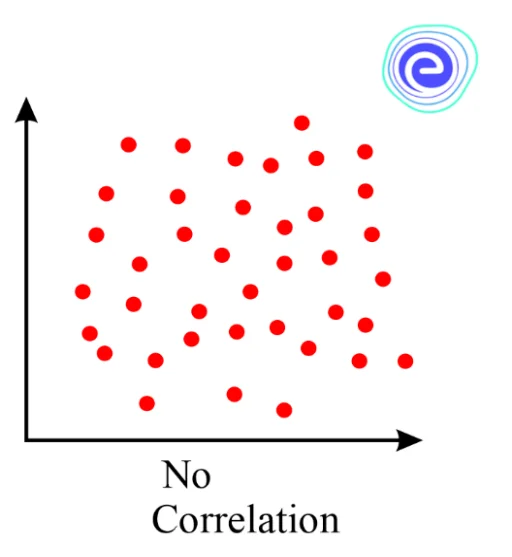

Pearson’s Correlation

Pearson’s correlation coefficient is the most common type of correlation coefficient. Pearson’s correlation (also known as Pearson’s \(r\)) is a correlation coefficient that is frequently used in linear regression.

The linear correlation coefficient, denoted by \(r\), defines the degree of relationship between two variables. It is known as the cross-correlation coefficient because it predicts the relationship between two variables.

If \(x\) and \(y\) are the two variables under consideration, the correlation coefficient can be computed using the formula.

\(r = \frac{{n\left( {\sum x y} \right) – \left( {\sum x } \right)\left( {\sum y } \right)}}{\sqrt{{\left[ {n\sum {{x^2}} – {{\left( {\sum x } \right)}^2}} \right]\left[ {n\sum {{y^2}} – {{\left( {\sum y } \right)}^2}} \right]}}}\)

Here,

\(n = \) number of values or elements

\(x = \) Sum of \({{\rm{1}}^{{\rm{st}}}}\) values list

\(y = \) Sum of \({{\rm{2}}^{{\rm{nd}}}}\) values list

\(xy = \) Sum of the product of \({{\rm{1}}^{{\rm{st}}}}\) and \({{\rm{2}}^{{\rm{nd}}}}\) values

\({x^2} = \) Sum of squares of \({{\rm{1}}^{{\rm{st}}}}\) values

\({y^2} = \) Sum of squares of \({{\rm{2}}^{{\rm{nd}}}}\) values

Solved Examples – Line of Regression

Below are a few solved examples that can help in getting a better idea:

Q.1. Find the linear regression equation for the data given below:

\(X\)	\(2\)	\(3\)	\(5\)	\(8\)
\(Y\)	\(3\)	\(6\)	\(5\)	\(12\)

Ans:

\(X\)	\(Y\)	\({X^2}\)	\(XY\)
\(2\)	\(3\)	\(4\)	\(6\)
\(3\)	\(6\)	\(9\)	\(18\)
\(5\)	\(5\)	\(25\)	\(25\)
\(8\)	\(12\)	\(64\)	\(96\)
\(\sum X = 18\)	\(\sum Y = 26\)	\({\sum X ^2} = 102\)	\(\sum X Y = 145\)

Linear regression equation is \(Y = a + bX\)
By using the formula, we will get the values of \(a\) and \(b\)
\(b = \frac{{n\sum x y – \left( {\sum x } \right)\left( {\sum y } \right)}}{{n\sum {{x^2}} – {{\left( {\sum x } \right)}^2}}}\)
\(b = \frac{{4 \times 145 – (18) \times (26)}}{{4 \times 102 – {{(18)}^2}}}\)
\( = \frac{{112}}{{84}}\)
\(\therefore \,b = 1.33\)
\(a = \frac{{\sum y – b\left( {\sum x } \right)}}{n}\)
\(a = \frac{{26 – 1.33 \times 18}}{4}\)
\(\therefore \,a = 0.515\)
Hence, the linear regression equation is \(Y = 0.515 + 1.33X\).

Q.2. For the following two sets of data, find a linear regression equation

\(x\)	\(2\)	\(4\)	\(6\)	\(8\)
\(y\)	\(3\)	\(7\)	\(5\)	\(10\)

Ans:

\(x\)	\(y\)	\({x^2}\)	\(xy\)
\(2\)	\(3\)	\(4\)	\(6\)
\(4\)	\(7\)	\(16\)	\(28\)
\(6\)	\(5\)	\(36\)	\(30\)
\(8\)	\(10\)	\(64\)	\(80\)
\(\Sigma x = 20\)	\(\Sigma y = 25\)	\(\Sigma {x^2} = 120\)	\(\Sigma xy = 144\)

The linear regression equation is \(Y = a + bX\)
By using the formula, we will get the values of \(a\) and \(b\)
\(b = \frac{{n\sum x y – \left( {\sum x } \right)\left( {\sum y } \right)}}{{n\sum {{x^2}} – {{\left( {\sum x } \right)}^2}}}\)
\(b = \frac{{4 \times 144 – (20) \times (25)}}{{4 \times 120 – {{(20)}^2}}} = \frac{{76}}{{80}} = 0.95\)
\(a = \frac{{\sum y – b\left( {\sum x } \right)}}{n}\)
\(a = \frac{{25 – 0.95 \times 20}}{4} = 1.5\)
Hence, the linear regression equation is \(Y = 1.5 + 0.95X\).

Q.3. Find the regression coefficients

Age	Glucose Level
\(43\)	\(99\)
\(21\)	\(65\)
\(25\)	\(79\)
\(42\)	\(75\)
\(57\)	\(87\)
\(59\)	\(81\)

Ans:

Age \((x)\)	Glucose Level \((y)\)	\(xy\)	\({x^2}\)
\(43\)	\(99\)	\(4257\)	\(1849\)
\(21\)	\(65\)	\(1365\)	\(441\)
\(25\)	\(79\)	\(1975\)	\(625\)
\(42\)	\(75\)	\(3150\)	\(1764\)
\(57\)	\(87\)	\(4959\)	\(3249\)
\(59\)	\(81\)	\(4779\)	\(3481\)
Total \(= 247\)	\(486\)	\(20485\)	\(11409\)

The regression equation is \(Y = a + bX\)
By using the formula, we will get the values of \(a\) and \(b\)
\(b = \frac{{n\sum x y – \left( {\sum x } \right)\left( {\sum y } \right)}}{{n\sum {{x^2}} – {{\left( {\sum x } \right)}^2}}}\)
\(b = \frac{{6 \times 20485 – (247) \times (486)}}{{6 \times 11409 – {{(247)}^2}}} = \frac{{2868}}{{7445}} = 0.385\)
\(a = \frac{{\sum y – b\left( {\sum x } \right)}}{n}\)
\(a = \frac{{486 – 0.385 \times 247}}{6} = 65.15\)
Hence, the linear regression equation is \(Y = {\rm{65}}{\rm{.15}} + {\rm{0}}{\rm{.385}}X\).

Q.4. Find the line of regression for the below data:

\(A\)	\(B\)
\(6.25\)	\(4.03\)
\(6.5\)	\(4.02\)
\(6.5\)	\(4.02\)
\(6\)	\(4.04\)
\(6.25\)	\(4.03\)
\(6.25\)	\(4.03\)

Ans:

\(X\)	\(Y\)	\(XY\)	\({X^2}\)
\(6.25\)	\(4.03\)	\(25.19\)	\(39.06\)
\(6.5\)	\(4.02\)	\(26.13\)	\(42.25\)
\(6.5\)	\(4.02\)	\(26.13\)	\(42.25\)
\(6\)	\(4.04\)	\(24.24\)	\(36\)
\(6.25\)	\(4.03\)	\(25.19\)	\(39.06\)
\(6.25\)	\(4.03\)	\(25.19\)	\(39.06\)
Total \( = 37.75\)	\(24.17\)	\(152.06\)	\(237.69\)

The line of regression is \(Y = a + bX\)
By using the formula, we will get the values of \(a\) and \(b\)
\(b = \frac{{n\sum x y – \left( {\sum x } \right)\left( {\sum y } \right)}}{{n\sum {{x^2}} – {{\left( {\sum x } \right)}^2}}}\)
\(b = \frac{{6 \times 152.06 – (37.75) \times (24.17)}}{{6 \times 237.69 – {{37.75}^2}}}\)
\(\therefore \,b = – 0.04\)
\(a = \frac{{\sum y – b\left( {\sum x } \right)}}{n}\)
\(a = \frac{{24.17 – ( – 0.04) \times 37.75}}{6}\)
\(\therefore \,a = 4.28\)
Hence, the line of regression is \(Y = – 0.04X + 4.28\)

Q.5. Find the Pearson’s coefficient for the given data

Age	Glucose Level
\(43\)	\(99\)
\(21\)	\(65\)
\(25\)	\(79\)
\(42\)	\(75\)
\(57\)	\(87\)
\(59\)	\(81\)

Ans:

Age \((x)\)	Glucose Level \((y)\)	\(xy\)	\({x^2}\)	\({Y^2}\)
\(43\)	\(99\)	\(4257\)	\(1849\)	\(9801\)
\(21\)	\(65\)	\(1365\)	\(441\)	\(4225\)
\(25\)	\(79\)	\(1975\)	\(625\)	\(6241\)
\(42\)	\(75\)	\(3150\)	\(1764\)	\(5625\)
\(57\)	\(87\)	\(4959\)	\(3249\)	\(7569\)
\(59\)	\(81\)	\(4779\)	\(3481\)	\(6561\)
Total \( = 247\)	\(486\)	\(20485\)	\(11409\)	\(40022\)

The Pearson’s correlation coefficient is given by
\(r = \frac{{n\left( {\sum x y} \right) – \left( {\sum x } \right)\left( {\sum y } \right)}}{\sqrt{{\left[ {n\sum {{x^2}} – {{\left( {\sum x } \right)}^2}} \right]\left[ {n\sum {{y^2}} – {{\left( {\sum y } \right)}^2}} \right]}}}\)
\(r\frac{{6 \times 20485 – (247 \times 486)}}{{\sqrt {\left[ {6 \times 11409 – {{(247)}^2}} \right]\left[ {6 \times 40022 – {{(486)}^2}} \right]} }}\)
\(\therefore \,r = 0.5298\)
Hence, the correlation coefficient is \({\rm{0}}{\rm{.5298}}\).

Summary

Linear regression is the most fundamental and widely used type of predictive analysis in statistics. Its entire concept is to investigate two things. First, determine whether a set of predictor variables accurately predicts an outcome.

Second, determine which variables, in particular, are significant predictors of the outcome variable and how.

These regression estimates are extremely helpful in explaining the relationship between one or more independent variables and one dependent variable. The linear equation is the most basic form. Correlation coefficients are used to assess the strength of a relationship between two variables.

Pearson’s correlation is a correlation coefficient that is frequently used in linear regression.

FAQs on Line of Regression

Students might be having many questions with respect to the Line of Regression. Here are a few commonly asked questions and answers.

Q.1. What does the line of a regression tell you?
Ans: The regression line depicts the relationship between the independent and dependent variables.

Q.2. How do you find a regression line?
Ans: The equation for a linear regression line is \(Y = a + bX\), where \(X\) is the explanatory variable and \(Y\) is the dependent variable. The slope of a line is \(b\), and the intercept (the value of \(y\) when \(x = 0\)) is \(a\).

Q.3. What is the regression line called?
Ans: The regression line is also known as the “line of best fit” because it is the line that fits the best when drawn through the points. It is a line that minimises the difference between actual and predicted scores.

Q.4. What are examples of linear regression?
Ans: The number of sales and the effect of fertiliser on the total crops, agricultural scientists use the linear regression. Doctors use to find the dosage and effect of the drug on blood pressure etc.

Q.5. What is the coefficient of correlation?
Ans: The correlation coefficient is a statistical concept that aids in establishing a relationship between the predicted and actual values from a statistical experiment.

We hope this information about the Line of Regression has been helpful. If you have any doubts, comment in the section below, and we will get back to you soon.

Stay tuned to embibe for the latest update on Line of Regression.