Methods of studying correlation: In everyday language, the term correlation refers to some kind of association. However, in statistical terms, correlation denotes the relationship between two quantitative variables. Correlation, in other words, is the strength of the linear relationship between two or more continuous variables.

If a change in one variable causes a corresponding change in the other variable, the two variables are correlated. Scatter diagrams, Karl Pearson’s coefficient of correlation, and Spearman’s rank correlation are three important tools for studying correlation. There are three types of correlation: based on the direction of change, based on the number of variables and based on the constancy of the ratio of change.

What Are the Different Types of Correlation?

We can classify the correlations based on the direction of change of variables, the number of variables studied and the constancy of the ratio change between the variables.

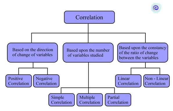
Type I: Based on the direction of change of variables

Correlation is classified into two types based on the direction of change of the variables: positive correlation and negative correlation.

• Positive Correlation:
  When the variables change in the same direction, the correlation is said to be positive. The sign of the positive correlation is \( + 1.\)
  Example: When income rises, so does consumption and when income falls, consumption does too.
• Negative Correlation:
  When the variables move in opposite directions, the correlation is negative. The sign of negative correlation is \( – 1.\)
  Example: Height above sea level and temperature are an example of a negative association. It gets colder as you climb the mountain (ascend in elevation) (decrease in temperature).

Type II: Based upon the number of variables studied

There are three types of correlation, based on the number of variables.

• Simple Correlation:
  The study of only two variables is referred to as simple correlation. The usage of fertilisers and paddy yield is an example of a simple connection, as paddy yield is dependent on fertiliser use.
• Multiple Correlation:
  Multiple correlations is defined as the study of three or more variables at the same time. Crimes in a city, for example, maybe influenced by illiteracy, growing population, and unemployment, among other factors.
• Partial Correlation:
  If there are three or more variables, but only two are considered while keeping the other variables constant, the correlation is said to be partial. For example, while controlling for weight and exercise, you would wish to investigate if there is a link between the amount of food consumed and blood pressure.

Type III: Based upon the constancy of the ratio of change between the variables

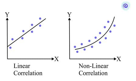
Correlation is classified into two types based on the consistency of the ratio of change between the variables: linear correlation and non-linear correlation.

• Linear Correlation:
  The correlation is said to be linear when the change in one variable bears a constant ratio to the change in the other.
  Example: \(Y = a + bx\)
• Non-Linear Correlation:
  If the change in one variable does not have a constant ratio to the change in the other variables, the correlation is non-linear.
  Example: \(Y = a + b{x^2}\)

PRACTICE EXAM QUESTIONS AT EMBIBE

Methods of Constructing Correlation

Scatter diagrams, Karl Pearson’s coefficient of correlation, and Spearman’s rank correlation are three important tools for studying correlation.

• A scatter diagram visually depicts the nature of an association without providing a numerical value.
• Karl Pearson’s correlation coefficient provides a numerical measure of the linear relationship between two variables. If a straight line can represent a relationship, it is said to be linear.
• Spearman’s correlation coefficient measures the linear relationship between the ranks assigned to individual items based on their attributes.

Scatter Diagram Method

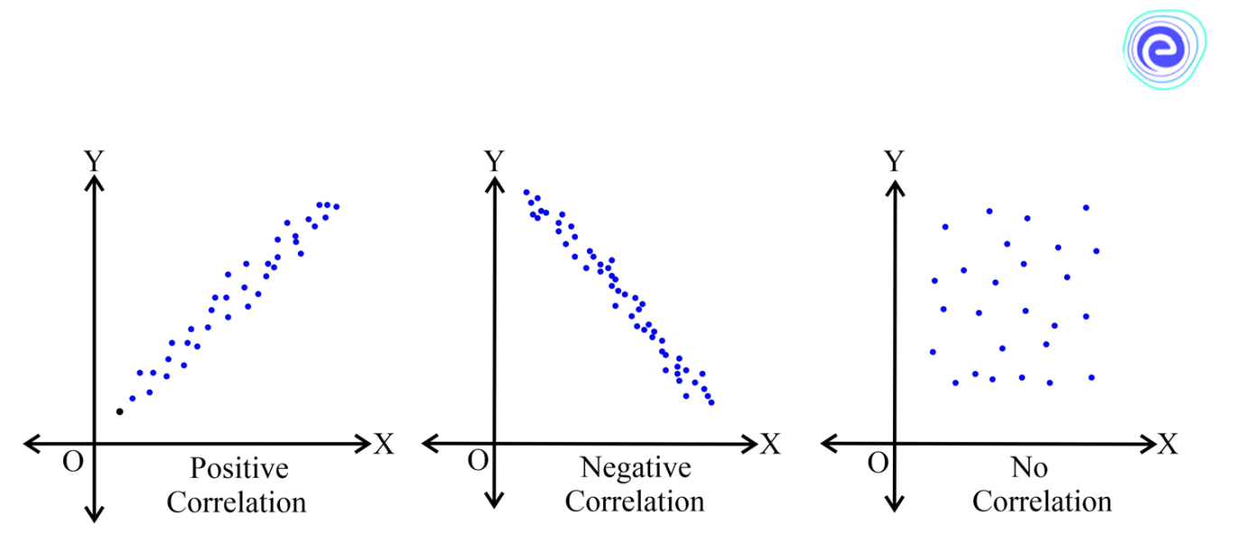
A scatter diagram is an effective method for visually examining the form of a relationship without calculating any numerical value. The values of these two variables are plotted as points on graph paper in this technique. A scatter diagram can provide a good indication of the nature of a relationship.

The degree of closeness of the scatter points and their overall direction in a scatter diagram allow us to examine their relationship. If the points fall on a straight line, the correlation is perfect and in unity. The correlation is low if the scatter points are widely dispersed around the line. If the scatter points are close to or on a line, the correlation is said to be linear.

Steps of plotting scatter diagram are follows.

• Step 1: Consider the graph (\(XY\) plane)
• Step 2: Consider the independent variable on the \(x\)-axis
• Step 3: Consider the dependent variable on the \(y\)-axis
• Step 4: Plot the various values of \(x\) and \(y\) on the graph.

If all values rise, there is a positive correlation; there is a negative correlation if they fall.

Karl Pearson’s Correlation Coefficient

Pearson’s correlation coefficient is a popular name for Karl Pearson’s method. This is also referred to as the product-moment correlation coefficient or the simple correlation coefficient. It provides a precise numerical value for the linear relationship between two variables \(X\) and \(Y.\)
Karl Pearson’s correlation coefficient should only be used when the variables have a linear relationship. It is calculated using the arithmetic mean and standard deviation. The correlation coefficient \(\left( r \right)\) is also called the linear correlation coefficient. It is a mathematical expression that measures the strength and direction of a linear relationship between two variables. The value of \(r\) ranges from \( – 1\) to \(1.\)
Karl Pearson’s correlation coefficient is calculated using the following formula:
\(r = \frac{{N\sum X Y – \left( {\sum X } \right)\left( {\sum Y } \right)}}{{\sqrt {N\sum {{X^2}} – {{\left( {\sum X } \right)}^2}} \sqrt {N\sum {{Y^2}} – {{\left( {\sum Y } \right)}^2}} }}\)
The value of the correlation coefficient is \( – 1 \leqslant r \leqslant 1.\) If the value of \(r\) is outside this range in any exercise, it indicates an error in calculation.

Spearman’s Coefficient of Rank Correlation

The formula is based on a simple correlation coefficient with individual values replaced by ranks. These rankings are used to calculate the correlation. This coefficient measures the linear association between the ranks assigned to these units rather than their values. Spearman’s rank correlation is a formula given below.
\(\rho = 1 – \frac{{6\sum {d_i^2} }}{{{n^3} – n}}\)
Here \(n\) is the number of observations, and \(d\) is the difference between the ranks assigned to one variable and those assigned to the other variable.

Interpretation of correlation coefficient

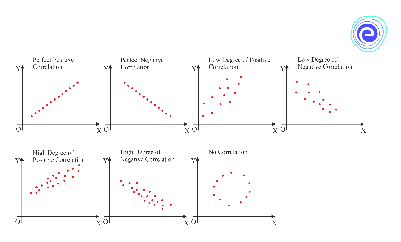
We know that the value of \(r\) ranges from \( – 1\) to \( +1.\) The sign of the correlation coefficient \(\left( { + ,\, – } \right)\) denotes whether the relationship is positive or negative. The correlation coefficient’s magnitude determines the strength of the relationship between the variables. The various \(‘r’\) value cut-offs and interpretations are listed below.

Correlation  value	Interpretation
\( + 1\)	perfect positive correlation
\( – 1\)	perfect negative correlation
\(0.0\)	no linear relationship
\(0.00\) to \(0.29\)	weak correlation
\(0.30\) to \(0.69\)	moderate correlation
\(0.70\) to \(1.00\)	high correlation

Solved Examples – Methods of Studying Correlation

Below are a few solved examples that can help in getting a better idea.

Q.1. Calculate and interpret Karl Pearson’s correlation coefficient based on the following data.

Price: \(X\)	\(10\)	\(12\)	\(14\)	\(15\)	\(19\)
Supply: \(Y\)	\(40\)	\(41\)	\(48\)	\(60\)	\(50\)

Ans:

Price: \(X\)	Supply: \(Y\)	\(XY\)	\({X^2}\)	\({Y^2}\)
\(10\)	\(40\)	\(400\)	\(100\)	\(1600\)
\(12\)	\(41\)	\(492\)	\(144\)	\(1681\)
\(14\)	\(48\)	\(672\)	\(196\)	\(2304\)
\(15\)	\(60\)	\(900\)	\(225\)	\(3600\)
\(19\)	\(50\)	\(950\)	\(361\)	\(2560\)
\(\sum X = 70\)	\(\sum Y = 239\)	\(\sum X Y = 3414\)	\(\sum {{X^2}} = 1026\)	\(\sum {{Y^2}} = 11685\)

Pearson’s correlation coefficient is given by
\(r = \frac{{N\sum X Y – \left( {\sum X \times \sum Y } \right)}}{{\sqrt {N\sum {{X^2}} – {{\left( {\sum Y } \right)}^2}} \times \sqrt {N\sum {{Y^2}} – {{\left( {\sum Y } \right)}^2}} }}\)
\( = \frac{{5 \times 3414 – \left( {70 \times 239} \right)}}{{\sqrt {5 \times 1026 – {{\left( {70} \right)}^3}} \times \sqrt {5 \times 11685 – {{\left( {239} \right)}^2}} }}\)
\( = \frac{{17,070 – 16,730}}{{\sqrt {230} \times \sqrt {1304} }}\)
\(\therefore r = 0.621\)
The price of the product and its supply are positively correlated. When the price of a product rises, so does the supply of that product.

Q.2. Estimate the coefficient of correlation for the following data using the actual mean method.

Years from purchase	\(3\)	\(6\)	\(8\)	\(9\)	\(10\)	\(6\)
Cost of annual increment	\(1\)	\(7\)	\(4\)	\(6\)	\(8\)	\(4\)

Ans:

\(X\)	\(X = x – \bar x\)	\({X^2}\)	\(y\)	\(Y = y – \bar y\)	\({Y^2}\)	\(XY\)
\(3\)	\( – 4\)	\(16\)	\(1\)	\( – 4\)	\(1\)	\(16\)
\(6\)	\( – 1\)	\(1\)	\(7\)	\( 2\)	\(49\)	\( – 2\)
\(8\)	\( +1\)	\(1\)	\(4\)	\( – 1\)	\(16\)	\( – 1\)
\(9\)	\( 2\)	\(4\)	\(6\)	\( 1\)	\(36\)	\( 2\)
\(10\)	\( 3\)	\(9\)	\(8\)	\( 3\)	\(64\)	\( 9\)
\(6\)	\( – 1\)	\(1\)	\(4\)	\( – 1\)	\(16\)	\( 1\)
\(\overline x = 7\)	\( 0\)	\( 32\)	\(\bar y = 7\)	\( 0\)	\(182\)	\( 25\)

Coefficient of correlation is given by \(r = \frac{{\sum x y}}{{\sqrt {\sum {{x^2}} \times \sum {{y^2}} } }},\) Where \(x = \Sigma \left( {X – \bar X} \right)y = \sum {\left( {Y – \bar Y} \right)} \)
\( = \frac{{25}}{{\sqrt {32} \times \sqrt {182} }}\)
\( = \frac{{25}}{{5.66 \times 13.49}}\)
\(\therefore r = 0.327\)
The car is getting older, and the cost of maintenance is rising. The age of a car and its maintenance are related in a positive way.

Q.3. Calculate the correlation coefficient and give their relationship.

\(X\)	\(-3\)	\(-2\)	\(-1\)	\(1\)	\(2\)	\(3\)
\(Y\)	\(9\)	\(4\)	\(1\)	\(1\)	\(4\)	\(9\)

Ans:

\(X\)	\(Y\)	\(XY\)	\({X^2}\)	\({Y^2}\)
\(-3\)	\(9\)	\(-27\)	\(9\)	\(81\)
\(-2\)	\(4\)	\(-8\)	\(4\)	\(16\)
\(-1\)	\(1\)	\(-1\)	\(1\)	\(1\)
\(1\)	\(1\)	\(1\)	\(1\)	\(1\)
\(2\)	\(4\)	\(8\)	\(4\)	\(16\)
\(3\)	\(9\)	\(27\)	\(9\)	\(81\)
\(\sum X = 0\)	\(\sum Y = 28\)	\(\sum X Y = 0\)	\(\sum {{X^2}} = 28\)	\(\sum {{Y^2}} = 196\)

Coefficeient of correlation is given by
\(r = \frac{{\sum X Y – \frac{{\sum X \times \Sigma Y}}{N}}}{{\sqrt {\sum {{X^2}} – \frac{{{{\left( {\sum X } \right)}^2}}}{N}} \sqrt {\sum {{Y^2}} – \frac{{{{\left( {\Sigma Y} \right)}^2}}}{N}} }}\)
\( = \frac{{0 – \frac{{0 \times 28}}{6}}}{{\sqrt {28 – \frac{{{{\left( {28} \right)}^2}}}{6}} \sqrt {196 – \frac{{{{\left( {196} \right)}^2}}}{6}} }}\)
\( = \frac{0}{{\sqrt {28 – \frac{{{{\left( {28} \right)}^2}}}{6}} \sqrt {196 – \frac{{{{\left( {196} \right)}^2}}}{6}} }}\)
\(\therefore r = 0\)
There is no linear correlation between \(X\) and \(Y\) because \(r\) is zero.

Q.4. Calculate the correlation coefficient and give their relationship.

\(X\)	\(1\)	\(3\)	\(4\)	\(5\)	\(7\)	\(8\)
\(Y\)	\(2\)	\(6\)	\(8\)	\(10\)	\(14\)	\(16\)

Ans:

\(X\)	\(Y\)	\(XY\)	\({X^2}\)	\({Y^2}\)
\(1\)	\(2\)	\(2\)	\(1\)	\(4\)
\(3\)	\(6\)	\(18\)	\(9\)	\(36\)
\(4\)	\(8\)	\(32\)	\(16\)	\(64\)
\(5\)	\(10\)	\(50\)	\(25\)	\(100\)
\(7\)	\(14\)	\(98\)	\(49\)	\(196\)
\(8\)	\(16\)	\(128\)	\(64\)	\(256\)
\(\sum X = 28\)	\(\sum Y = 56\)	\(\sum X Y = 328\)	\(\sum {{X^2}} = 164\)	\(\sum {{Y^2}} = 656\)

Coefficeient of correlation is given by
\(r = \frac{{\sum X Y – \frac{{\sum X \times \Sigma Y}}{N}}}{{\sqrt {\sum {{X^2}} – \frac{{{{\left( {\sum X } \right)}^2}}}{N}} \sqrt {\sum {{Y^2}} – \frac{{{{\left( {\sum Y } \right)}^2}}}{N}} }}\)
\( = \frac{{328 – \frac{{56 \times 28}}{6}}}{{\sqrt {164 – \frac{{{{\left( {28} \right)}^2}}}{6}} \sqrt {656 – \frac{{{{\left( {56} \right)}^2}}}{6}} }}\)
\( = \frac{{328 – \frac{{1568}}{6}}}{{\sqrt {164 – \frac{{784}}{6}\sqrt {656 – \frac{{3136}}{6}} } }}\)
\( = \frac{{328 – 261.33}}{{\sqrt {164 – 130.67} \times \sqrt {656 – 522.67} }}\)
\( = \frac{{66.67}}{{\sqrt {33.33} \sqrt {133.33} }}\)
\( = \frac{{66.67}}{{66.67}}\)
\(\therefore r = 1\)
Because the correlation coefficient between the two variables is \(1,\) they are in perfect positive correlation.

Q.5. Explain the values of the coefficient of correlation as \( – 1,0\) and \(1.\)
Ans:
The explanations for the values of coefficient of correlation are:
1. If \(r = 0,\) the two variables are uncorrelated. There is no logical connection between them. However, other types of relationships may exist, and thus the variables may not be independent.
2. If \(r = 1,\) the correlation is \(100\% \) positive. The relationship is exact because if one rises, the other rises in the same proportion, and if one falls, the other falls in the same proportion.
3. When \(r = -1,\) the correlation is completely negative. It has an exact relationship: if one increases, the other decreases in the same proportion, and if one decreases, the other increases in the same proportion.

Summary

Correlation investigates and quantifies the direction and strength of relationships between variables. The scatter diagram visually represents a relationship that is not limited to linear relationships. The linear relationship between variables is measured by Karl Pearson’s coefficient of correlation and Spearman’s rank correlation. When the variables cannot be precisely measured, rank correlation can be used.

However, these measures do not imply causation. Correlation knowledge allows us to predict the direction and intensity of change in a variable when the correlated variable changes. Positive, negative, zero, simple, multiple, partial, linear, and non-linear correlations are some of the frequently used types of correlations.

FAQs on Methods of Studying Correlation

Students might be having many questions with respect to the Methods of Studying Correlation. Here are a few commonly asked questions and answers.

Q.1. What are the \(3\) types of correlation?
Ans: A correlational study can gives three types of components: a positive correlation, a negative correlation, or no correlation.

Q.2. Which is a method of measuring correlation?
Ans: The Pearson correlation method, which assigns a value between \( – 1\) and \(1,\) is the most commonly used method for numerical variables.

Q.3. What is the simplest method of studying correlation?
Ans: The scatter diagram method is a simple method for determining the relationship between variables.

Q.4. Which are the two methods of correlation?
Ans: Pearson’s product-moment coefficient of correlation and scatter diagram methods are two main methods to calculate the correlation.

Q.5. Is it possible to measure any relationship using a simple correlation coefficient?
Ans: No, only a linear relationship can be measured by a simple correlation coefficient.

ATTEMPT MOCK TESTS ON EMBIBE

We hope this information about the Methods of Studying Correlation has been helpful. If you have any doubts, comment in the section below, and we will get back to you soon.