


Ellipse: Do you know the orbit of planets, moon, comets, and other heavenly bodies are elliptical? Mathematics defines an ellipse as a plane curve surrounding...
Last Modified 14-04-2025

Harvest Smarter Results!
Celebrate Baisakhi with smarter learning and steady progress.
Unlock discounts on all plans and grow your way to success!

Ellipse: Definition, Properties, Applications, Equation, Formulas
April 14, 2025
Altitude of a Triangle: Definition & Applications
April 14, 2025
Manufacturing of Sulphuric Acid by Contact Process
April 13, 2025
Refining or Purification of Impure Metals
April 13, 2025
Pollination and Outbreeding Devices: Definition, Types, Pollen Pistil Interaction
April 13, 2025
Acid Rain: Causes, Effects
April 10, 2025
Congruence of Triangles: Definition, Properties, Rules for Congruence
April 8, 2025
Complementary and Supplementary Angles: Definition, Examples
April 8, 2025
Nitro Compounds: Types, Synthesis, Properties and Uses
April 8, 2025
Bond Linking Monomers in Polymers: Biomolecules, Diagrams
April 8, 2025
Operations on matrices: This rectangular arrangement of numbers in columns and rows, called a matrix, has varied applications in real life. Its applications range from optics to electrical circuits in the field of Science and from solving linear equations to graphical representation in Mathematics. Matrices are also employed to encrypt data, study the trends of shares, in seismic surveys, and make animation more accurate.
Similar to real numbers, arithmetic operations can also be performed on matrices. The following operations can be carried out on matrices.
Read this article further to know how these operations are performed with a suitable explanation and examples.

Two matrices can be added if and only if they have the same order. In simpler words, to add two matrices, they must have the same number of rows and columns.
While adding two matrices, add the corresponding entries in the given matrices. The number of addition operations is equal to the number of elements in each of the matrices. For two matrices \(A\) and \(B\) of the order \(2 \times 2\), their addition is defined as,
\(\,\left[ {\begin{array}{*{20}{c}} a&b \\ c&d\end{array}} \right]\, + \left[ {\begin{array}{*{20}{c}} w&x \\ y&z\end{array}} \right] = \,\left[ {\begin{array}{*{20}{c}}{\left( {a + w} \right)}&{\left( {b + x} \right)} \\{\left( {c + y} \right)}&{\left( {d + z} \right)}\end{array}} \right]\)
As we know, only matrices of the same order can be added. The addition of matrices of different orders is undefined.
\(\left[ {\begin{array}{*{20}{c}} p&q \\ \begin{gathered}r \hfill \\ t \hfill \\\end{gathered} &\begin{gathered} s \hfill \\ u \hfill \\\end{gathered} \end{array}} \right]\, + \,\left[ {\begin{array}{*{20}{c}}i&j \\k&l\end{array}} \right]\)
Here, the order of \(\left[ {\begin{array}{*{20}{c}} p&q \\ \begin{gathered} r \hfill \\ t \hfill \\\end{gathered} &\begin{gathered} s \hfill \\ u \hfill \\\end{gathered} \end{array}} \right]\,\) is \(3 \times 2\), and that of \(\left[ {\begin{array}{*{20}{c}} i&j \\ k&l\end{array}} \right]\) is \(2 \times 2\). Hence, these two matrices cannot be added.
Two matrices \(A\) and \(B\) of the same order, \(m \times n\), can be added in any way, and the resulting matrix will remain unchanged.
\(A + B = B + A\)
Proof:
Let \(A = \left[ {{a_{ij}}} \right],\,B = \left[ {{b_{ij}}} \right]\)
Then, \(A + B = \left[ {{a_{ij}}} \right] + \left[ {{b_{ij}}} \right]\)
\(\left[ {{a_{ij}} + {b_{ij}}} \right]\)
Since the addition of numbers is commutative,
\(A + B = \left[ {{b_{ij}} + {a_{ij}}} \right]\)
\( = \left[ {{b_{ij}}} \right] + \left[ {{a_{ij}}} \right]\)
\(\therefore A + B = B + A\)
Hence proved that matrices are commutative under addition.
2. Associative Law
For the addition of three matrices \(A,B\), and \(C\) of the same order, \(m \times n\), the associative property is defined as,
\(A + \left( {B + C} \right) = \left( {A + B} \right) + C\)
Proof:
Let \(A = \left[ {{a_{ij}}} \right],\,B = \left[ {{b_{ij}}} \right],\,C = \left[ {{c_{ij}}} \right]\)
Then, \(A + \left( {B + C} \right) = \left[ {{a_{ij}}} \right] + \left( {\left[ {{b_{ij}}} \right] + \left[ {{c_{ij}}} \right]} \right)\)
\( = \left[ {{a_{ij}}} \right] + \left( {\left[ {{b_{ij}}} \right] + \left[ {{c_{ij}}} \right]} \right)\)
\(= \left[ {{a_{ij}}} \right] + \left[ {{b_{ij}} + {c_{ij}}} \right]\)
\(= \left[ {{a_{ij}} + \left( {{b_{ij}} + {c_{ij}}} \right)} \right]\)
Since the addition of numbers is associative,
\(A + \left( {B + C} \right) = \left[ {\left( {{a_{ij}} + {b_{ij}}} \right) + {c_{ij}}} \right]\)
\( = \left[ {{a_{ij}} + {b_{ij}}} \right] + \left[ {{c_{ij}}} \right]\)
\( = \left( {\left[ {{a_{ij}}} \right] + \left[ {{b_{ij}}} \right]} \right) + \left[ {{c_{ij}}} \right]\)
\(\therefore A + \left( {B + C} \right) = \,\,\,\left( {A + B} \right) + C\)
Hence proved that matrices are associative under addition.
3. Additive Identity
For a matrix \(P\) of the order \(m \times n\), there exists a matrix \(O\) of the same order, such that,
\(P + O = O + P = P\)
Here, \(O\) is the zero matrix of the same order \(m \times n\), and is called the additive identity.
Example:
Consider the matrix \(A = \,\left[ {\begin{array}{*{20}{c}}0&1&0 \\2&3&1 \\1&0&1\end{array}} \right]\)
Let \(O = \,\left[ {\begin{array}{*{20}{c}} 0&0&0 \\ 0&0&0 \\ 0&0&0\end{array}} \right]\) be the identity matrix.
Then,
\(A + O = \left[ {\begin{array}{*{20}{c}} 0&1&0 \\ 2&3&1 \\ 1&0&1\end{array}} \right] + \left[ {\begin{array}{*{20}{c}} 0&0&0 \\ 0&0&0 \\ 0&0&0\end{array}} \right]\)
\( = \left[ {\begin{array}{*{20}{c}} {0 + 0}&{1 + 0}&{0 + 0} \\ {2 + 0}&{3 + 0}&{1 + 0} \\ {1 + 0}&{0 + 0}&{1 + 0}\end{array}} \right]\)
\( = \,\left[ {\begin{array}{*{20}{c}} 0&1&0 \\ 2&3&1 \\ 1&0&1\end{array}} \right]\)
\(\therefore A + O = A\)
4. Additive Inverse
There exists a unique matrix \(-A\) for every matrix \(A\), such that,
\(A + \left( { – A} \right) = O\)
Here, \(O\) is a zero matrix of the order \(m \times n\), and \(-A\) is called the additive inverse of \(A\) or the negative of \(A\).
Similar to the addition of matrices, subtraction is also performed on the corresponding entries of the two matrices. This is also called the difference of matrices.
\(\left[ {\begin{array}{*{20}{c}}a&b \\c&d\end{array}} \right]\, – \left[ {\begin{array}{*{20}{c}}w&x \\y&z\end{array}} \right] = \,\left[ {\begin{array}{*{20}{c}} {\left( {a – w} \right)}&{\left( {b – x} \right)} \\ {\left( {c – y} \right)}&{\left( {d – z} \right)}\end{array}} \right]\)
Difference of matrices can also be written as,
\(\,\left[ {\begin{array}{*{20}{c}} a&b \\ c&d\end{array}} \right]\, – \left[ {\begin{array}{*{20}{c}} w&x \\ y&z\end{array}} \right] = \left[ {\begin{array}{*{20}{c}}a&b \\c&d\end{array}} \right]\, + \left( { – 1} \right)\,\left[ {\begin{array}{*{20}{c}} w&x \\ y&z\end{array}} \right]\)
\(\therefore \,\left[ {\begin{array}{*{20}{c}} a&b \\ c&d\end{array}} \right]\, – \left[ {\begin{array}{*{20}{c}} w&x \\ y&z\end{array}} \right] = \left[ {\begin{array}{*{20}{c}} a&b \\ c&d\end{array}} \right]\, + \,\left[ {\begin{array}{*{20}{c}} { – w}&{ – x} \\ { – y}&{ – z}\end{array}} \right]\)
Simply put, the difference of two matrices \(A\) and \(B\) is \(A-B\), and can be written as the sum of matrix \(A\) and the matrix \(-B\).
\(A – B = A + \left( { – B} \right)\)
Apart from the addition and subtraction of matrices, the other common operation performed is the multiplication of a matrix by a constant called a scalar.
While multiplying a scalar with a matrix, the number is multiplied with every element in the matrix.
Let \(A = \left[ {\begin{array}{*{20}{c}} {{a_{11}}}&{{a_{12}}}&{{a_{13}}} \\{{b_{11}}}&{{b_{12}}}&{{b_{13}}} \\{{c_{11}}}&{{c_{12}}}&{{c_{13}}}\end{array}} \right]\)and the scalar be \(p\). Then, \(p \times A\) is given by,
\(p \times A = p \times \left[ {\begin{array}{*{20}{c}}{{a_{11}}}&{{a_{12}}}&{{a_{13}}} \\{{b_{11}}}&{{b_{12}}}&{{b_{13}}} \\{{c_{11}}}&{{c_{12}}}&{{c_{13}}}\end{array}} \right]\)
\(\therefore p \times A = \left[ {\begin{array}{*{20}{c}} {p{a_{11}}}&{p{a_{12}}}&{p{a_{13}}} \\ {p{b_{11}}}&{p{b_{12}}}&{p{b_{13}}} \\ {p{c_{11}}}&{p{c_{12}}}&{p{c_{13}}}\end{array}} \right]\)
In line with the associative property, that of scalar multiplication of matrices is given by,
\(\left( {xy} \right)A = x\left( {yA} \right)\)
We know that the scalar is multiplied with every element in the matrix, and associative property holds for numbers. Hence, the scalar multiplication of a matrix is associative.
2. Distributive Law
Let \(A,\) and \(B\) be the matrices, \(x,\) and \(y\) be the scalars. The distributive property of scalar multiplication of matrices is defined as,
\(x\left( {A + B} \right) = xA + xB\)
\(\left( {x + y} \right)A = xA + yA\)
3. Multiplicative Identity
The scalar, when multiplied by a matrix \(A,\) results in the same matrix \(A\) is called the multiplicative identity.
\(1 \cdot A = A\)
The multiplicative identity of scalar multiplication of a matrix is \(1\).
4. Multiplying by a Zero
Similar to multiplying a number by \(0\), multiplying a matrix \(A\) by \(0\) also results in a zero.
\(0 \times A = 0\)
Similarly, the scalar product of a zero matrix is always a zero matrix.
\(c \times 0 = 0\)
Here, \(0\) is a zero matrix of the order \(m \times n\), and \(c \ne 0\).
5. Scalar Multiplication as Repeated Addition
Scalar multiplication of a matrix is nothing but repeated addition of the matrix by itself \(n\) times, where \(n\) is the scalar.
Illustration:
If \(A=\left[ {\begin{array}{*{20}{c}} 2&5 \\ 7&3\end{array}} \right]\), find \(A + A + A + A\).
Solution:
\(A + A + A + A = \left[ {\begin{array}{*{20}{c}} 2&5 \\ 7&3\end{array}} \right] + \left[ {\begin{array}{*{20}{c}} 2&5 \\ 7&3\end{array}} \right] + \left[ {\begin{array}{*{20}{c}} 2&5 \\ 7&3\end{array}} \right] + \left[ {\begin{array}{*{20}{c}} 2&5 \\ 7&3\end{array}} \right]\)
\( = \left[ {\begin{array}{*{20}{c}} {2 + 2 + 2 + 2}&{5 + 5 + 5 + 5} \\ {7 + 7 + 7 + 7}&{3 + 3 + 3 + 3}\end{array}} \right]\)
\( = \left[ {\begin{array}{*{20}{c}} 8&{20} \\ {21}&{12}\end{array}} \right]\)
\( = \left[ {\begin{array}{*{20}{c}} {4 \cdot 2}&{4 \cdot 5} \\ {4 \cdot 7}&{4 \cdot 3} \end{array}} \right]\)
\( = 4\left[ {\begin{array}{*{20}{c}} 2&5 \\ 7&3\end{array}} \right]\)
\(A + A + A + A = \,\,4 \times A\)
Hence, proved that scalar multiplication is repeated addition.

As we have learnt to multiply a matrix by a scalar, let us now learn to multiply two matrices.
Two matrices can be multiplied if and only if they have the same inner order. In simpler words, to multiply two matrices, the number of columns in the first matrix must be equal to the number of rows in the second matrix.
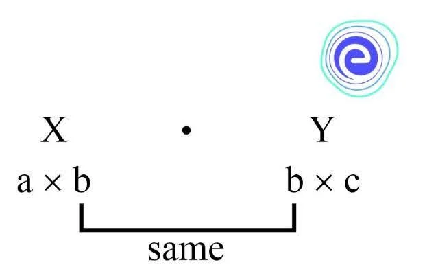
The order of the product matrix will have the order \(a \times c\).
Multiplication of two matrices involves several calculations. Before we begin the long process, let us start small and learn to multiply a row matrix and a column matrix.
Consider the column matrix \(A = \left[ \begin{gathered} 2 \hfill \\ 3 \hfill \\ 4 \hfill \\\end{gathered} \right]\) and the row matrix \(B = \left[ {6\,\,\,4\,\,\,3} \right]\). Note that the number of rows in \(A\) and the number of columns in \(B\) are equal.
\(A \times B = \left[ \begin{gathered} 2 \hfill \\ 3 \hfill \\ 4 \hfill \\\end{gathered} \right]\,\, \times \,\,\left[ {6\,\,\,4\,\,\,3} \right]\)
To multiply a row matrix and a column matrix, we multiply the corresponding elements as shown below.
\(\,\left[ \begin{gathered} {a_{11}} \hfill \\ {a_{21}} \hfill \\ {a_{31}} \hfill \\\end{gathered} \right]\,\, \times \,\,\left[ {{b_{11}}\,\,\,{b_{12}}\,\,\,{b_{13}}} \right] = \left[ {\begin{array}{*{20}{c}}{{a_{11}} \times {b_{11}}}&{{a_{11}} \times {b_{12}}}&{{a_{11}} \times {b_{13}}} \\ {{a_{21}} \times {b_{11}}}&{{a_{21}} \times {b_{12}}}&{{a_{21}} \times {b_{13}}} \\ {{a_{31}} \times {b_{11}}}&{{a_{31}} \times {b_{12}}}&{{a_{31}} \times {b_{13}}}\end{array}} \right]\)
Thus, the resulting matrix will have the number of rows from \(A\) and the number of columns from \(B\) as \(3 \times 3\).
\(\therefore \left[ \begin{gathered} 2 \hfill \\ 3 \hfill \\ 4 \hfill \\\end{gathered} \right] \times \left[ {6\,\,\,4\,\,\,3} \right] = \left[ {\begin{array}{*{20}{c}} {2 \times 6}&{2 \times 4}&{2 \times 3} \\ {3 \times 6}&{3 \times 4}&{3 \times 3} \\ {4 \times 6}&{4 \times 4}&{4 \times 3}\end{array}} \right]\)
\(A \times B = \left[ {\begin{array}{*{20}{c}} {12}&8&6 \\ {18}&{12}&9 \\ {24}&{16}&{12}\end{array}} \right]\)
Similarly, we can multiply a row matrix with a column matrix.
\(B \times A = \left[ {6\,\,\,4\,\,\,3} \right] \times \left[ \begin{gathered}2 \hfill \\3 \hfill \\4 \hfill \\\end{gathered} \right]\)
The multiplication is carried out as shown below.
\(\left[ {{b_{11}}\,\,\,{b_{12}}\,\,\,{b_{13}}} \right]\, \times \,\left[ \begin{gathered} {a_{11}} \hfill \\ {a_{21}} \hfill \\ {a_{31}} \hfill \\\end{gathered} \right] = \left[ {{b_{11}}\left( {{a_{11}}} \right) + {b_{12}}\left( {{a_{21}}} \right) + {b_{13}}\left( {{a_{31}}} \right)} \right]\)
Observe that the resulting matrix will have the number of rows from \(B\) and the number of columns from \(A\) as \(1 \times 1\).
\(\left[ {\begin{array}{*{20}{c}}
6&4&3
\end{array}} \right] \times \left[ {\begin{array}{*{20}{c}}
2 \\
3 \\
4
\end{array}} \right] = \left[ {\left( {6 \times 2} \right) + \left( {4 \times 3} \right) + \left( {3 \times 4} \right)} \right]\)
\( = \left[ {12 + 12 + 12} \right]\)
\(\therefore \,B \times A = \left[ {36} \right]\)
This is called the dot product, and it is the exact method we will follow to calculate the elements in the product matrix while multiplying larger matrices.
Multiply \(A = \left[ {\begin{array}{*{20}{c}} 1&2&{ – 1} \\ 3&2&0 \\ { – 4}&0&2\end{array}} \right]\) and \(B = \left[ {\begin{array}{*{20}{c}} 3&4&2 \\ 0&1&0 \\ { – 2}&0&1\end{array}} \right]\)
Here, observe that the order of \(A\) is \(3 \times 3\) and that of \(B\) is also \(3 \times 3\). Hence, the order of the product matrix is \(3 \times 3\).
Let \(\left[ {\begin{array}{*{20}{c}} {{e_{11}}}&{{e_{12}}}&{{e_{13}}} \\ {{e_{21}}}&{{e_{22}}}&{{e_{23}}} \\ {{e_{31}}}&{{e_{32}}}&{{e_{33}}}\end{array}} \right]\)be the \(3 \times 3\) product matrix.
Now, let’s find each of the elements in the product matrix using the dot product method.
| \({e_{11}} = \left[ {1\,\,\,2\,\,\, – 1} \right] \times \left[ \begin{gathered} 3 \hfill \\ 0 \hfill \\ – 2 \hfill \\\end{gathered} \right]\) \( = \left[ {\left( {1 \times 3} \right) + \left( {2 \times 0} \right) + \left( { – 1 \times – 2} \right)} \right]\) \( = \left[ {3 + 0 + 2} \right]\) \(\therefore {e_{11}} = \left[ 5 \right]\) | \({e_{12}} = \left[ {1\,\,\,2\,\,\, – 1} \right] \times \left[ \begin{gathered} 4 \hfill \\ 1 \hfill \\ 0 \hfill \\\end{gathered} \right]\) \( = \left[ {\left( {1 \times 4} \right) + \left( {2 \times 1} \right) + \left( { – 1 \times 0} \right)} \right]\) \( = \left[ {4 + 2 + 0} \right]\) \(\therefore {e_{21}} = \left[ 6 \right]\) | \({e_{13}} = \left[ {1\,\,\,2\,\,\, – 1} \right] \times \left[ \begin{gathered} 2 \hfill \\ 0 \hfill \\ 1 \hfill \\\end{gathered} \right]\) \( = \left[ {\left( {1 \times 2} \right) + \left( {2 \times 0} \right) + \left( { – 1 \times 1} \right)} \right]\) \( = \left[ {2 + 0 – 1} \right]\) \(\therefore {e_{13}} = \left[ 1 \right]\) |
| \({e_{21}} = \left[ {3\,\,\,2\,\,\,0} \right] \times \left[ \begin{gathered} 3 \hfill \\ 0 \hfill \\ – 2 \hfill \\\end{gathered} \right]\) \( = \left[ {\left( {3 \times 3} \right) + \left( {2 \times 0} \right) + \left( {0 \times – 2} \right)} \right]\) \( = \left[ {9 + 0 + 0} \right]\) \(\therefore {e_{21}} = \left[ 9 \right]\) | \({e_{22}} = \left[ {3\,\,\,2\,\,\,0} \right] \times \left[ \begin{gathered} 4 \hfill \\ 1 \hfill \\ 0 \hfill \\\end{gathered} \right]\) \( = \left[ {\left( {3 \times 4} \right) + \left( {2 \times 1} \right) + \left( {0 \times 0} \right)} \right]\) \( = \left[ {12 + 2 + 0} \right]\) \(\therefore {e_{22}} = \left[ 14 \right]\) | \({e_{23}} = \left[ {3\,\,\,2\,\,\,0} \right] \times \left[ \begin{gathered} 2 \hfill \\ 0 \hfill \\ 1 \hfill \\ \end{gathered} \right]\) \( = \left[ {\left( {3 \times 2} \right) + \left( {2 \times 0} \right) + \left( {0 \times 1} \right)} \right]\) \( = \left[ {6 + 0 + 0} \right]\) \(\therefore {e_{23}} = \left[ 6 \right]\) |
| \({e_{31}} = \left[ {-4\,\,\,0\,\,\,2} \right] \times \left[ \begin{gathered} 3 \hfill \\ 0 \hfill \\ – 2 \hfill \\\end{gathered} \right]\) \( = \left[ {\left( {-4 \times 3} \right) + \left( {0 \times 0} \right) + \left( {2 \times – 2} \right)} \right]\) \( = \left[ {-12 + 0 -4} \right]\) \(\therefore {e_{31}} = \left[ -16 \right]\) | \({e_{32}} = \left[ {-4\,\,\,0\,\,\,2} \right] \times \left[ \begin{gathered} 4 \hfill \\ 1 \hfill \\ 0 \hfill \\\end{gathered} \right]\) \( = \left[ {\left( {-4 \times 4} \right) + \left( {0 \times 1} \right) + \left( {2 \times 0} \right)} \right]\) \( = \left[ {-16 + 0 +0} \right]\) \(\therefore {e_{32}} = \left[ -16 \right]\) | \({e_{33}} = \left[ {-4\,\,\,0\,\,\,2} \right] \times \left[ \begin{gathered} 2 \hfill \\ 0 \hfill \\ 1 \hfill \\\end{gathered} \right]\) \( = \left[ {\left( {-4 \times 2} \right) + \left( {0 \times 0} \right) + \left( {2 \times 1} \right)} \right]\) \( = \left[ {-8 + 0 +2} \right]\) \(\therefore {e_{33}} = \left[ -6 \right]\) |
These individual elements can be arranged to form the resultant product matrix.
\(\therefore \left[ {\begin{array}{*{20}{c}} 1&2&{ – 1} \\ 3&2&0 \\ { – 4}&0&2\end{array}} \right] \times \,\left[ {\begin{array}{*{20}{c}} 3&4&2 \\ 0&1&0 \\ { – 2}&0&1\end{array}} \right] = \left[ {\begin{array}{*{20}{c}} 5&6&1 \\ 9&{14}&6 \\ { – 16}&{ – 16}&{ – 6}\end{array}} \right]\)
Note that the bigger the matrix, the more extensive is the calculation involved in multiplying them.
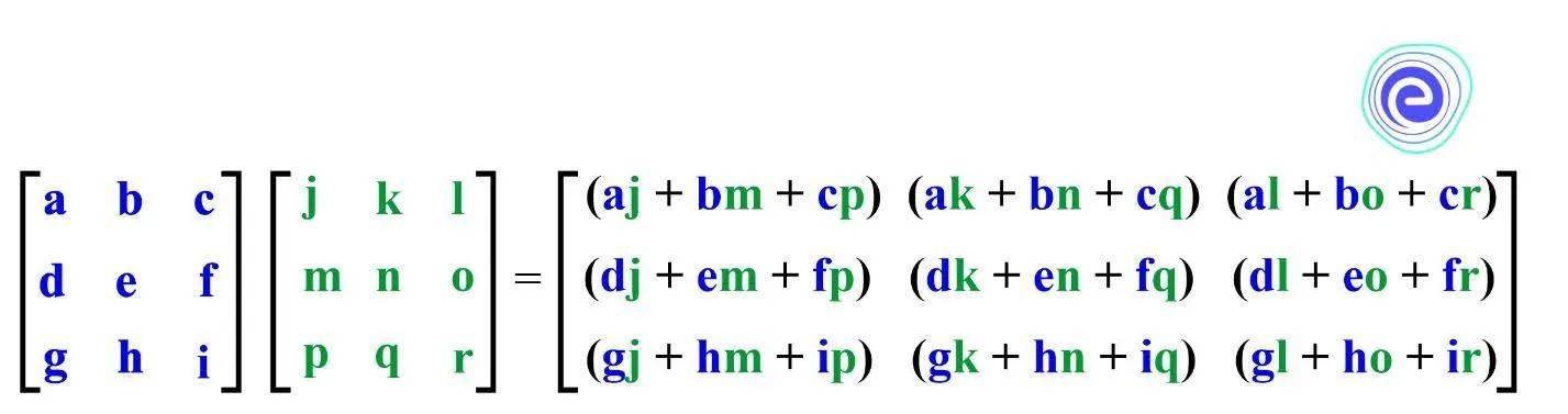
The formula for \(3 \times 3\) multiplication is as given below.
As discussed earlier in this article, we have seen that the product of a row matrix and a column matrix is not the same as that of a column matrix and row matrix.
\(\left[ \begin{gathered} 2 \hfill \\ 3 \hfill \\ 4 \hfill \\\end{gathered} \right] \times \left[ {6\,\,\,4\,\,\,3} \right] \ne \,\,\,\left[ {6\,\,\,4\,\,\,3} \right] \times \,\left[ \begin{gathered} 2 \hfill \\ 3 \hfill \\ 4 \hfill \\\end{gathered} \right]\)
\(\left[ {\begin{array}{*{20}{c}} {12}&8&6 \\ {18}&{12}&9 \\ {24}&{16}&{12}\end{array}} \right] \ne \left[ {36} \right]\)
\(A \cdot B \ne B \cdot A\)
Hence, matrix multiplication is not commutative.
For any three matrices \(A, B\), and \(C\) associative law is defined as,
\(A \cdot \left( {B \cdot C} \right) = \left( {A \cdot B} \right) \cdot C\)
Observe that the associative law does not change the order of multiplication of the matrices but alters only the association. We first multiply the two matrices that are associated, and then multiply the third matrix to the product matrix.
Matrix multiplication is associative.
For any three matrices \(A, B\), and \(C\) distributive law is defined as,
\(A\left( {B + C} \right) = AB + AC\)
\(\left( {A + B} \right)C = AC + BC\)
Observe that in both the equations, the order of multiplication of the matrices is preserved.
Matrix multiplication is distributive.
When multiplied by a \(0\), we know that any number results in a \(0\). Similarly, when a matrix is multiplied by a zero matrix, the result will be a zero matrix. But this property states that when multiplying some non-zero matrices, the product may be a zero matrix.
For two non-zero matrices \(A\) and \(B\),
\(A \cdot B = 0\)
Example:
Let \(A = \left[ {\begin{array}{*{20}{c}}0&{ – 1} \\0&2\end{array}} \right]\) and \(B = \left[ {\begin{array}{*{20}{c}}3&5 \\0&0\end{array}} \right]\)
Then,
\(A \cdot B = \left[ {\begin{array}{*{20}{c}} 0&{ – 1} \\ 0&2\end{array}} \right]\,\left[ {\begin{array}{*{20}{c}} 3&5 \\ 0&0\end{array}} \right]\)
\( = \left[ {\begin{array}{*{20}{c}} 0&0 \\0&0\end{array}} \right]\)
\(A \cdot B = 0\)
Therefore, we can say that the product of two matrices can still be a zero matrix even the matrices that are multiplied are non-zero.
Note: This does not hold for numbers. The product of two non-zero numbers can never be a zero.
For a square matrix \(X\), and identity matrix \(I\) of the same order,
\(X \cdot I = I \cdot X = X\)
Q.1. Find the additive inverse of \(\left[ {\begin{array}{*{20}{c}} 1&4 \\ 5&3 \end{array}} \right]\)
Sol: Let, \(A= \left[ {\begin{array}{*{20}{c}} 1&4 \\ 5&3 \end{array}} \right]\)
We know that, \(A + \left( { – A} \right) = 0\)
\( – A = 0 – A\)
\(\therefore – A = \left[ {\begin{array}{*{20}{c}} 0&0 \\ 0&0 \end{array}} \right] – \left[ {\begin{array}{*{20}{c}} 1&4 \\ 5&3 \end{array}} \right]\)
\( \Rightarrow – A = \left[ {\begin{array}{*{20}{c}} { – 1}&{ – 4} \\ { – 5}&{ – 3} \end{array}} \right]\)
Q.2. Solve \(\left( {\begin{array}{*{20}{c}} 2&1 \\ 1&2\end{array}} \right)\,\left( \begin{gathered} x \hfill \\ y \hfill \\\end{gathered} \right) = \left( \begin{gathered} 4 \hfill \\ 5 \hfill \\\end{gathered} \right)\)
Sol:
\(\left( {\begin{array}{*{20}{c}} 2&1 \\ 1&2\end{array}} \right)\,\left( \begin{gathered} x \hfill \\ y \hfill \\\end{gathered} \right) = \left( \begin{gathered} 4 \hfill \\ 5 \hfill \\\end{gathered} \right)\)
By matrix multiplication,
\(\left( \begin{gathered} 2x + y \hfill \\ x + 2y \hfill \\\end{gathered} \right) = \left( \begin{gathered} 4 \hfill \\ 5 \hfill \\\end{gathered} \right)\)
Rewriting as equations, we get,
\(2x + y = 4\) ………..\(1\)
\(x + 2y = 5\) …………\(2\)
Solving, we get,
\(y=2\)
Using \(\left( 1 \right) – 2 \times \left( 2 \right)\) we get,
\(2x + y = 4\)
\(2x + 4y = 10\)
\(-3y=-6\)
\(y=2\)
Substituting \(y=2\) in \(1\), we get,
\(x=1\)
Q.3. Simplify: \(\cos \theta \,\left[ {\begin{array}{*{20}{c}}{\cos \theta }&{\sin \theta } \\{ – \sin \theta }&{\cos \theta }\end{array}} \right]\, + \sin \theta \,\left[ {\begin{array}{*{20}{c}} {\sin \theta }&{ – \cos \theta } \\ {\cos \theta }&{\,\sin \,\theta }\end{array}} \right]\)
Sol:
Step 1: Perform scalar multiplication
\( = \,\left[ {\begin{array}{*{20}{c}} {{{\cos }^2}\theta }&{\sin \theta\, \cos \theta } \\ { – \sin \theta \,\cos \theta }&{{{\cos }^2}\theta }\end{array}} \right]\, + \,\left[ {\begin{array}{*{20}{c}} {{{\sin }^2}\theta }&{ – \sin \,\theta \,\cos \theta } \\ {\sin \,\theta \,\cos \theta }&{\,{{\sin }^2}\,\theta }\end{array}} \right]\)
Step 2: Perform addition of matrices
\( = \,\left[ {\begin{array}{*{20}{c}} {{{\cos }^2}\theta + \,{{\sin }^2}\theta }&{\sin \theta \cos \theta – \sin \theta \cos \theta } \\ { – \sin \theta \,\cos \theta + \sin \theta \cos \theta }&{{{\cos }^2}\theta + {{\sin }^2}\theta }\end{array}} \right]\)
Step 3: Simplify
\(\cos \theta \,\left[ {\begin{array}{*{20}{c}}{\cos \theta }&{\sin \theta } \\{ – \sin \theta }&{\cos \theta }\end{array}} \right]\, + \sin \theta \,\left[ {\begin{array}{*{20}{c}} {\sin \theta }&{ – \cos \theta } \\ {\cos \theta }&{\,\sin \,\theta }\end{array}} \right]\)
\( \Rightarrow \,\cos \theta \,\left[ {\begin{array}{*{20}{c}} {\cos \theta }&{\sin \,\theta \,} \\ { – \sin \,\theta \,}&{\,\cos \theta }\end{array}} \right] + \sin \,\theta \,\left[ {\begin{array}{*{20}{c}} {\sin \theta }&{ – \cos \,\theta \,} \\ {\cos \,\theta \,}&{\,\sin \theta }\end{array}} \right] = \left[ {\begin{array}{*{20}{c}} 1&{0\,} \\ {0\,}&{\,1}\end{array}} \right]\)
\(\therefore \,\,\cos \theta \,\left[ {\begin{array}{*{20}{c}} {\cos \theta }&{\sin \,\theta \,} \\ { – \sin \,\theta \,}&{\,\cos \theta }\end{array}} \right] + \sin \,\theta \,\left[ {\begin{array}{*{20}{c}}{\sin \theta }&{ – \cos \,\theta \,} \\ {\cos \,\theta \,}&{\,\sin \theta }\end{array}} \right] = {\text{Unit}}\,{\text{matrix}}\)
Q.4. Prove commutativity of matrix addition of \(X = \left[ \begin{gathered} 0\,\,\,\,\,3\,\,\,\,\,1 \hfill \\ 4\,\,\,\,\,7\,\,\,\,\,1 \hfill \\\end{gathered} \right]\) and \(Y = \left[ \begin{gathered} 1\,\,\,\,\,2\,\,\,\,\,1 \hfill \\ 1\,\,\,\,\,3\,\,\,\,\,2 \hfill \\\end{gathered} \right]\).
Sol:
\(X + Y = \left[ \begin{gathered} 0\,\,\,\,\,3\,\,\,\,\,1 \hfill \\ 4\,\,\,\,\,7\,\,\,\,\,1 \hfill \\\end{gathered} \right] + \left[ \begin{gathered} 1\,\,\,\,\,2\,\,\,\,\,1 \hfill \\ 1\,\,\,\,\,3\,\,\,\,\,2 \hfill \\\end{gathered} \right] = \left[ \begin{gathered} 1\,\,\,\,\,5\,\,\,\,\,2 \hfill \\ 5\,\,\,\,\,10\,\,\,3 \hfill \\\end{gathered} \right]\)
\(Y + X = \left[ \begin{gathered} 1\,\,\,\,\,2\,\,\,\,\,1 \hfill \\ 1\,\,\,\,\,3\,\,\,\,\,2 \hfill \\\end{gathered} \right] + \left[ \begin{gathered} 0\,\,\,\,\,3\,\,\,\,\,1 \hfill \\ 4\,\,\,\,\,7\,\,\,\,\,1 \hfill \\\end{gathered} \right] = \left[ \begin{gathered} 1\,\,\,\,\,5\,\,\,\,\,2 \hfill \\5\,\,\,\,\,10\,\,\,3 \hfill \\\end{gathered} \right]\)
\( \Rightarrow X + Y = Y + X\)
Q.5. Prove associativity of matrix addition using \(\left[ {\begin{array}{*{20}{c}} 1&7 \\ 4&5\end{array}} \right] + \left[ {\begin{array}{*{20}{c}} 3&8 \\ 7&4\end{array}} \right] + \left[ {\begin{array}{*{20}{c}}2&5 \\7&3\end{array}} \right]\)
Sol:
\(\left( {\left[ {\begin{array}{*{20}{c}} 1&7 \\ 4&5\end{array}} \right] + \left[ {\begin{array}{*{20}{c}} 3&8 \\ 7&4\end{array}} \right]} \right) + \left[ {\begin{array}{*{20}{c}} 2&5 \\ 7&3\end{array}} \right] = \left[ {\begin{array}{*{20}{c}} 1&7 \\ 4&5\end{array}} \right] + \left( {\left[ {\begin{array}{*{20}{c}} 3&8 \\ 7&4\end{array}} \right] + \left[ {\begin{array}{*{20}{c}} 2&5 \\ 7&3\end{array}} \right]} \right)\)
\(\left( {\left[ {\begin{array}{*{20}{c}} 4&{15} \\ {11}&9\end{array}} \right]} \right) + \left[ {\begin{array}{*{20}{c}} 2&5 \\ 7&3\end{array}} \right] = \left[ {\begin{array}{*{20}{c}} 1&7 \\ 4&5\end{array}} \right] + \left( {\left[ {\begin{array}{*{20}{c}} 5&{13} \\ {14}&7\end{array}} \right]} \right)\)
\(\left[ {\begin{array}{*{20}{c}} 6&{20} \\ {18}&{12}\end{array}} \right] = \left[ {\begin{array}{*{20}{c}} 6&20 \\ {18}&{12}\end{array}} \right]\)
Similar to real numbers, arithmetic operations can also be performed on matrices. The operations are addition, subtraction, multiplication of two matrices, and multiplication of a matrix by a scalar. To add or subtract two matrices, the operation is performed on the corresponding entries in the two matrix operands. Hence, they can be performed on matrices that have the same order. To multiply two matrices, their inner order must be equal. This means that the number of columns in the first matrix and the number of rows in the second must be the same. When multiplying a scalar, it is multiplied with every element in the matrix. The various properties of these operations are listed and explained.

Q.1. What are the operations on matrices?
Ans: Basic operations such as addition, subtraction, and multiplication can be carried out using matrices.
Q.2. What are the rules of matrices?
Ans: Rules of addition and multiplication of matrices:
| Commutative law of matrix addition | \(A + B = B + A\) |
| Associative law of matrix addition | \(A + \left( {B + C} \right) = \left( {A + B} \right) + C\) |
| Associative law of matrix multiplication | \(A + \left( {B + C} \right) = \left( {A + B} \right) + C\) |
| Distributive law of matrix multiplication | \(A\left( {B + C} \right) = AB + AC\) |
Q.3. Do matrices commute?
Ans: Matrices are commutative under addition, but they are not commutative under multiplication.
Q.4. Can you square a matrix?
Ans: To square a matrix, the matrix is multiplied by itself. Matrix multiplication can be carried out between two matrices where the number of columns in the first matrix is equal to the number of rows in the second matrix. Hence, we can square a matrix as long as it is a square matrix.
Q.5. Can you divide matrices?
Ans: Mathematically, there is no such thing as a division with matrices, unlike real numbers. Although we can say that when you multiply a matrix with a scalar \(\frac{1}{{x’}}\), where \(x\) is any real number, is called scalar division of matrices.
Learn the Properties of Matrix
We hope this detailed article on Operations on Matrices was helpful. If you have any doubts, let us know in the comment section below. Our team will get try to solve your queries at the earliest.


