Physical and geometrical interpretation of derivative: All functions with two variables can be represented by a graph on a two-dimensional plane, but we may not always draw it. It is interesting to visualise what the graph of the function would look like, i.e. we are always interested in finding out the behaviour of the curve of the function.

The qualitative study of the differential coefficient approximates the nature of the curve and its various properties. For example, monotonic nature, maxima/minima, and curvature. The derivative is the slope of the function’s graph at the point \((x,\,y)\), i.e. the slope of the tangent to the curve at the point \((x,\,y)\). So, the value of derivatives at point \(x\) on the curve can be used to determine the tangent to the curve at that point \(x\).

LEARN EXAM CONCEPTS ON EMBIBE

Physical Significance

Since \(\frac{{f\left( x \right) – f\left( a \right)}}{{x – a}}\) is an average rate of change of \(f(x)\) w.r.t \(x\) in \([a,\,x]\), therefore \(x \to a\) in the interval \([a,\,x]\) denotes an instant and \(\mathop {{\text{lim}}}\limits_{x \to a} \frac{{f\left( x \right) – f\left( a \right)}}{{x – a}}\) becomes the instantaneous rate of change of \(f(x)\) w.r.t \(x\) at \(x = a\). So, differentiability physically signifies no sudden change in the instantaneous rate of change at \(x = a\).

Geometrical Significance

Differentiability of \(f(x)\) at \(x = a\), implies \(LHD = RHD\). This, geometrically, means that a unique tangent with a finite slope can be drawn at \(x = a\) Therefore, the graph of \(f(x)\) must be smooth without any sharp corners at \(x = a\), and the tangent line at \(x = a\) is not vertical.

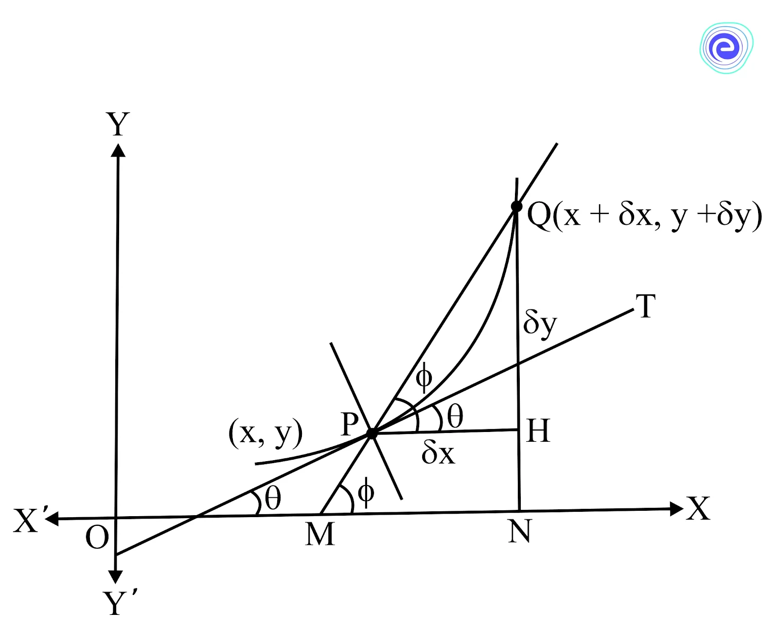
Given \(y = f(x)\) be a continuous curve and \(P(x,\,y)\) and \(Q\left( {x + \delta x,y + \delta y} \right)\) be any two points on this curve. Let \(Q\) be a point very near to \(P\). Let \(PT\) be the tangent to the curve at \(P\), which makes an angle \(\theta\) with the positive direction of \(x\)-axis and \(PQ\) cut \(OX\) at \(M\), so the angle \(\angle QMN = \phi\).

From \(Q\), draw a perpendicular \(QN\) on \(x\)-axis and from \(P\), draw \(PH\) perpendicular to \(QN\), respectively.

When \(Q\) approaches point \(P\), the chord \(QP\) rotates clockwise and tends to become the tangent at \(P\). (i.e., \(PT\)).

Also, when \(Q \to P\), then \(QH = \delta Y \to 0\) and \(PH = \delta x \to 0\).

Therefore \(\tan\, \phi = \frac{{QH}}{{PH}} = \frac{{\delta Y}}{{\delta X}}\) tends to \(\frac {0}{0}\) form.

Also, \(\phi \to \theta \) and therefore, \(\tan \theta = \mathop {\lim }\limits_{\delta x \to 0} \frac{{\delta y\;}}{{\delta x}}\) (popularly known as \(\frac {dy}{dx}\))

The derivative of \(y = f(x)\) at \(x = c\), geometrically represents the existence of a tangent (whether able to draw a unique tangent at that point) at \(P(c,\,f(c))\).

Now, conversely, the existence of the limit \(\phi \;\left( { – \frac{\pi }{2} < \phi < \frac{\pi }{2}} \right)\) implies the existence of a finite derivative \(f'(c)\).

PRACTICE EXAM QUESTIONS AT EMBIBE

Geometrical Interpretation of Partial Derivatives

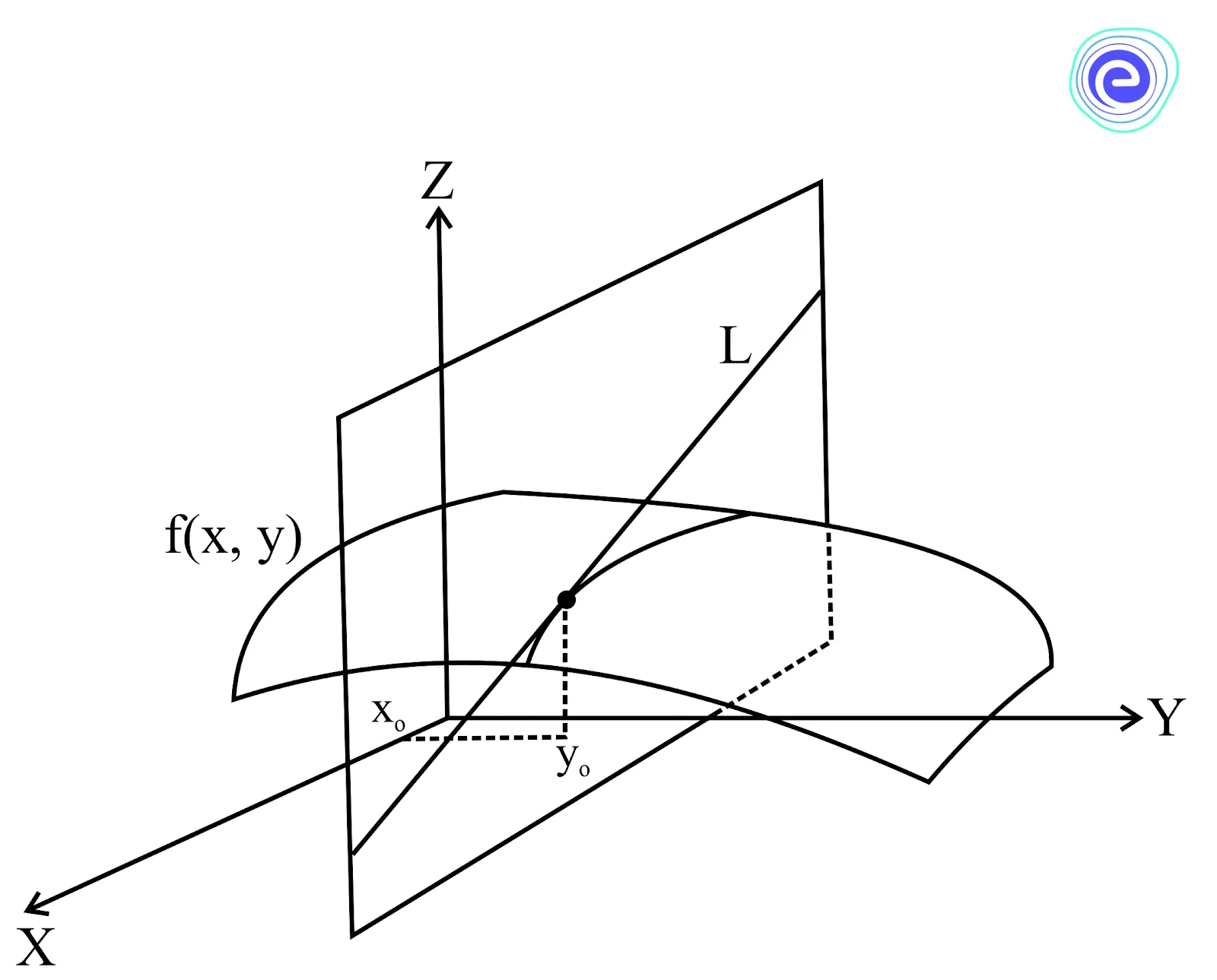
The meaning of the partial derivative at any given point \((a,\,b)\) is the value of the partial with respect to \(x\) i.e. \(f_x (a,\,b)\) is the slope of the tangent line to the intersection of the graph of \(f\) with the plane \(y = b\) at any point \((a,\,b)\). In other words, we can say that it shows how fast \(z\) changes with respect to the changes in \(x\).

Similarly, the value of \(f_y (a,\,b)\), is the slope of the tangent line to the intersection of the graph of \(f\) with the plane \(x = a\), i.e. the rate of change of \(z\) with respect to \(y\).

Geometrical Interpretation of Vector Derivative

The vector derivative is a derivative taken with respect to the vector field. Vector derivatives have a very important role in Physics, where they arise throughout fluid mechanics, magnetism, electricity, elasticity, and other areas of theoretical and applied Physics.

The vector derivatives can be combined in different ways, producing sets of identities that are also very important in Physics.

Differentiation of Vector-valued Functions

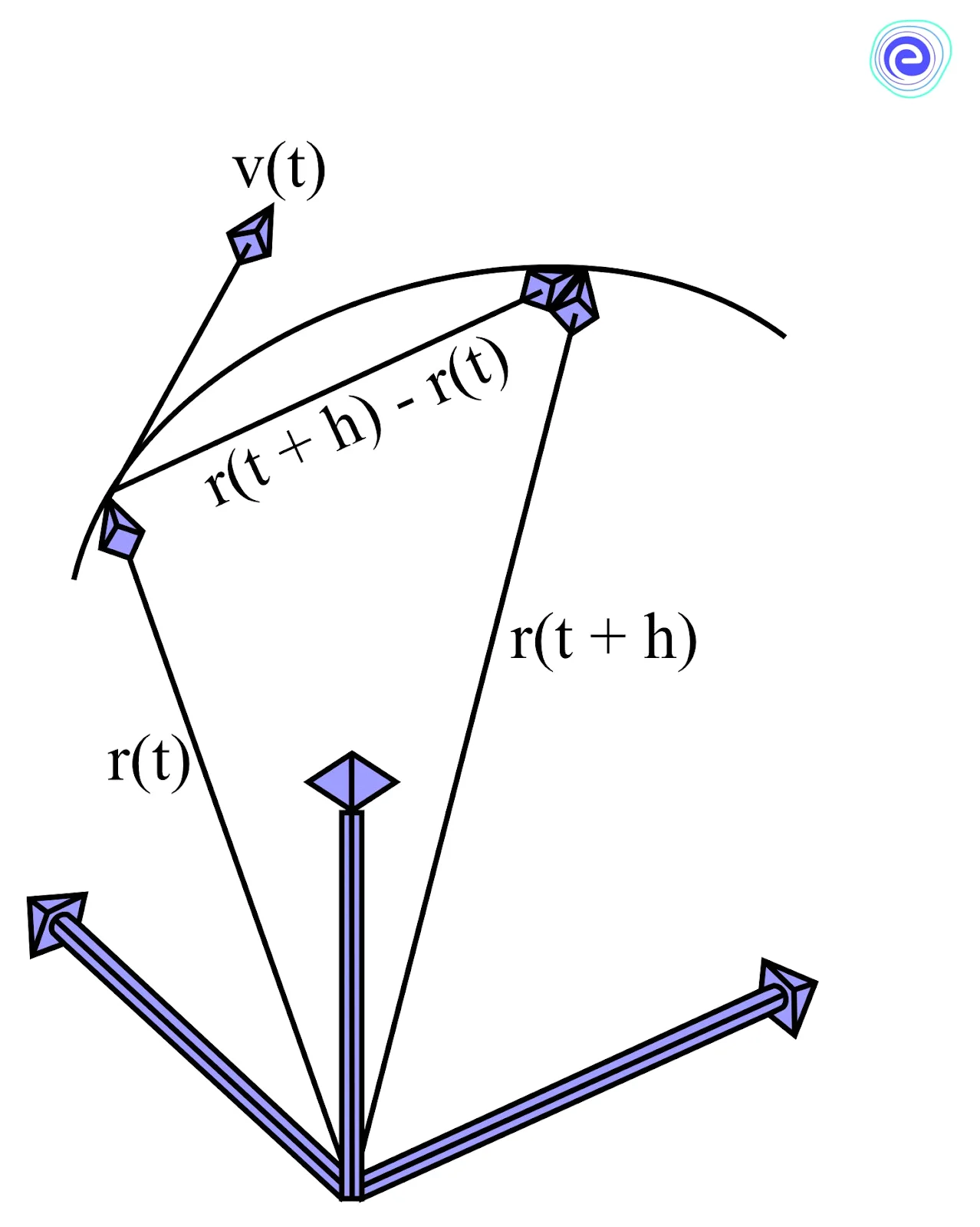
Let the curve \(C\), defined by \(r = r(t)\), be the vector-valued function of one variable. Let us imagine that \(C\) is the path taken by a particle in time \(t\). The vector \(r(t)\) is the position vector of the particle at time \(t\), and \(r(t + h)\) is the position vector at time \(t + h\). Then, the average velocity of the particle in the time interval \([t,\,t + h]\) is given by

\(\frac{{displacement\;vector}}{{lenth\;of\;time\;vector}}\; = \frac{{r\left( {t + h} \right) – r\left( t \right)}}{h}\)

In terms of the components of \(r\) this is

\(\left( {\frac{{x\left( {t + h} \right) – x\left( t \right)}}{h},\frac{{y\left( {t + h} \right) – y\left( t \right)}}{h},\frac{{z\left( {t + h} \right) – z\left( t \right)}}{h}} \right)\)

If each of the scalar functions \(x,\,y\) and \(z\) are differentiable, then this vector has a limit

\(\left( {\frac{{dx}}{{dt}},\frac{{dy}}{{dt}},\frac{{dz}}{{dt}}} \right) = \left( {x’,\;y’,\;z’} \right)\)

That is the instantaneous velocity of the particle \(v(t)\), i.e., if the motion is smooth, then

\(v\left( t \right) = \mathop {\lim }\limits_{h \to 0} \frac{{r\left( {t + h} \right) – r\left( t \right)}}{h} = \frac{d}{{dt}}r\left( t \right) = r’\left( t \right)\).

This vector lies along the tangent to the curve at \(r\) and has a length \(v\left( t \right)\; = \left| {V\left( t \right)} \right|\) is the instantaneous speed of the particle.

Similarly, we define the acceleration,

\(a\left( t \right) = \frac{d}{{dt}}v\left( t \right) = \frac{{{d^2}}}{{d{t^2}\;}}r\left( t \right) = r”\left( t \right)\).

More generally, for any curve \(r =r(\alpha)\) parametrised by \(\alpha\), the vector

\(\vec T = \frac{{dr}}{{d\alpha }}\)

is called the tangent vector to the curve, and the unit vector given by

\(\hat T = \frac{T}{{\left| T \right|}},\)

is called the unit tangent vector.

Different Types of Derivatives of Vectors

We already know about the derivatives and the partial derivatives of the scalar functions. Let us now discuss the other different types of “derivatives” of scalar and the vector functions.

Note: The result can be a scalar or vector function in the differentiation of scalar and vector functions.

If \(u,\,v,\,w\) are vectors and \(\alpha\) is a scalar, then several different products can be made.

Name of Product	Formula	Type of Result
Scalar multiplication	\(\alpha u\)	Vector
Scalar or dot product	\(u,\,v\)	Scalar
Vector or cross product	\(u \times v\)	Vector

Now, consider the vector differential operator

\(\nabla = \left( {\frac{\partial }{{\partial x}},\frac{\partial }{{\partial y}},\frac{\partial }{{\partial z}}} \right)\)

\(\nabla\) is read as \(del\) and is often confused with \(\Delta\), the capital Greek letter delta. One can form products of this vector with other vectors and scalars. Since it is an operator, it has to be the first term for the product to make sense.

For example, if \(f\) is a scalar field, we can form the scalar multiple with \(\nabla\) as the first term.

\(\nabla f = \left( {\frac{\partial }{{\partial x}},\frac{\partial }{{\partial y}},\frac{\partial }{{\partial z}}} \right)f = \left( {\frac{{\partial f}}{{\partial x}},\frac{{\partial f}}{{\partial y}},\frac{{\partial f}}{{\partial z}}} \right)\).

The result is a vector.

The following table summarises the names and notations for various vector derivatives with definitions and derivatives.

Vector Derivative	Symbol	Definition	Derivatives
Gradient	\(\nabla\)	The gradient of a scalar field \(f\) to be defined as \(\nabla f\)	\(grad\;f = \nabla f \) \(= \left( {\frac{{\partial f}}{{\partial x}},\frac{{\partial f}}{{\partial y}},\frac{{\partial f}}{{\partial z}}} \right)\)
Direction derivatives	\(\nabla_u\)	The rate of change of any scalar field \(f\) in the direction of a unit vector \(u = (u_1,\,u_2,\,u_3)\)	\(\frac{{\partial f}}{{\partial u}} = u \cdot \nabla f \) \(= {u_1}\frac{{\partial f}}{{\partial x}} + {u_2}\frac{{\partial f}}{{\partial y}} + {u_3}\frac{{\partial f}}{{\partial z}}\)
Divergence of a vector field	\(\nabla \cdot \)	The divergence of a vector field \(F = (F_1,\,F_2,\,F_3)\) is the scalar obtained as the scalar product of \(\nabla\) and \(F\)	\(div\;F = \nabla \cdot F =\) \(\frac{{\partial {F_1}}}{{\partial x}} + \frac{{\partial {F_2}}}{{\partial y}} + \frac{{\partial {F_3}}}{{\partial z}}\)
Laplacian of a scalar field	\(\nabla^2\)	For a given scalar field \(f\), \(grad\,f = {\nabla} f\) is a vector field, and the divergence of \({\nabla} f\) is the Laplacian of \(f\), written as \({\nabla}^2 f\)	\({\nabla ^2}f = \nabla \cdot \left( {\nabla f} \right) \) \(= \frac{{{\partial ^2}f}}{{\partial {x^2}}} + \frac{{{\partial ^2}f}}{{\partial {y^2}}} + \frac{{{\partial ^2}f}}{{\partial {z^2}}}\)
Curl of a vector field	\(\nabla \times\)	The curl of a vector field \(F = (F_1,\,F_2,\,F_3)\) is the vector obtained as the vector product of \(\nabla\) and \(F\).	\(curl\;F = \nabla \times F\) \( = \left( {\frac{{\partial {F_3}}}{{\partial y}} – \frac{{\partial {F_2}}}{{\partial z}}} \right)i\) \(+ \left( {\frac{{\partial {F_1}}}{{\partial z}} – \frac{{\partial {F_3}}}{{\partial x}}} \right)j + \left( {\frac{{\partial {F_2}}}{{\partial x}} – \frac{{\partial {F_1}}}{{\partial y}}} \right)k\)

Solved Examples – Physical and Geometrical Interpretation of Derivative

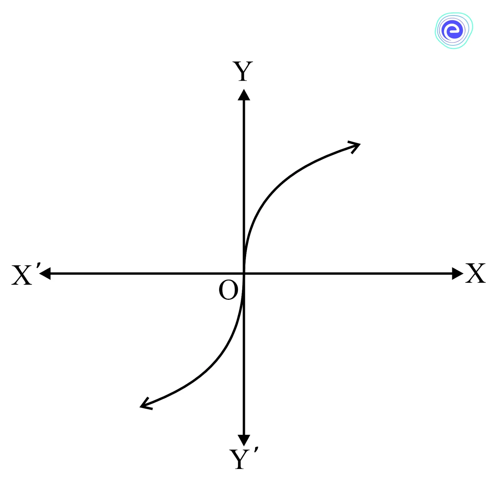
Q.1. Check the differentiability of \(f\left( x \right) = {x^{\frac{1}{3}}}\) at \(x = 0\)
Ans:
\(f’\left( 0 \right) = \mathop {\lim }\limits_{x \to 0} \frac{{({x^{\frac{1}{3}}} – 0)}}{{x – 0}} = \mathop {\lim }\limits_{x \to 0} \frac{1}{{{x^{\frac{2}{3}}}}} = \infty \)
\(f\) has a vertical directed tangent at \(x = 0\)
\(f\) is not differentiable at \(x = 0\)
See the graph of \(f\left( x \right) = {x^{\frac{1}{3}}}\)

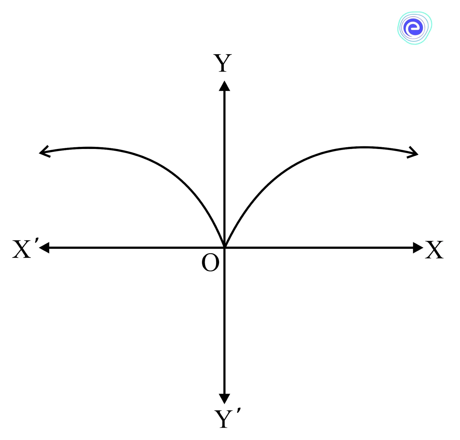
Q.2. Check the differentiability of \(f\left( x \right) = {x^{\frac{2}{3}}}\) at \(x = 0\)
Ans:
\(Lf’\left( 0 \right) = \mathop {\lim }\limits_{x \to {0^ – }} \frac{{{x^{\frac{2}{3}}} – 0}}{{x – 0}}\)
\( = \mathop {\lim }\limits_{x \to {0^ – }} {\left( {\frac{1}{x}} \right)^{\frac{1}{3}}}\)
\(\therefore \,Lf’\left( 0 \right) = – \infty \)
\(Rf’\left( 0 \right) = \infty \)
\(f\) has two vertical directed tangents to two branches at \(x = 0\)
\(f\) is not differentiable at \(x = 0\)

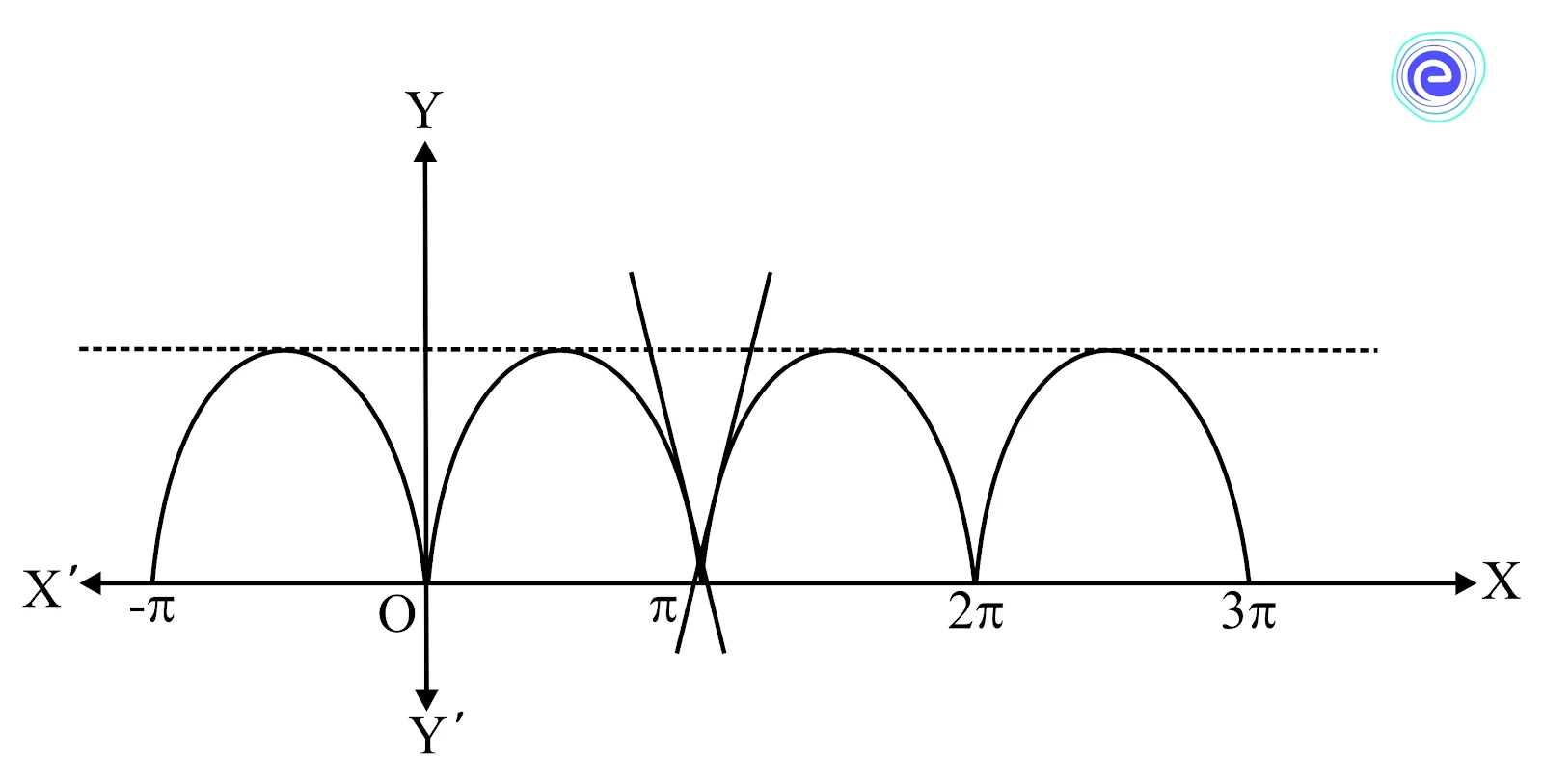
Q.3. Find all non-differentiable points of \(y = \left| {\sin x} \right|\).
Ans:
\(y = \left| {\sin x} \right|\), clearly, it is not differentiable when \(\sin x = 0,\, \Rightarrow x = n\pi ,\,n \in z\)

Q.4. Check the differentiability of \(f\left( x \right) = \left| {\ln x} \right|\) at \(x = 1\).
Ans:

\(f\left( x \right) = \left| {\ln x} \right| = \left\{ {\begin{array}{*{20}{c}} {\ln x\;if\ln x \geqslant 0 \Rightarrow x \geqslant 1} \\ { – \ln x\;\;if\ln x < 0 \Rightarrow 0 < x < 1} \end{array}} \right.\)

\(f’\left( {{1^ + }} \right) = \mathop {\lim }\limits_{h \to 0} \frac{{f\left( {1 + h} \right) – f\left( 1 \right)}}{h}\)
\( = \mathop {\lim }\limits_{h \to 0} \frac{{\ln \left( {1 + h} \right) – 0}}{h} = 1\)
\(f’\left( {{1^ – }} \right) = \mathop {\lim }\limits_{h \to 0} \frac{{f\left( {1 – h} \right) – f\left( 1 \right)}}{h}\)
\(= \mathop {\lim }\limits_{h \to 0} \frac{{ – \ln \left( {1 – h} \right) – 0}}{{ – h}} = – 1\)
Therefore, \(f\) is not differentiable at \(x = 1\).

Q.5. Examine the function, \(f\left( x \right) = x.\frac{{{a^{\frac{1}{x}}} – {a^{ – \frac{1}{x}}}}}{{{a^{\frac{1}{x}}} + {a^{ – \frac{1}{x}}}}},\,x \ne 0\) \((a > 0)\) and \(f(0) = 0\) for continuity and existence of the derivative at the origin.
Ans:
If \(a \in \left( {0,\,1} \right)\) then \(f’\left( {{0^ + }} \right) = – 1,\;f’\left( {{0^ – }} \right) = 1\)
Function is continuous but not derivable.
If \(a = 1; f(x) = 0\) is a constant \(\Rightarrow\) continuous, and derivable
If \(a > 1 f'(0^-) = -1; f'(0^+) = 1 \Rightarrow\) continuous but not derivable.

Summary

Differentiability physically signifies there is no sudden change in the instantaneous rate of change at \(x = a\). Differentiability of \(f(x)\) at \(x = a\), implies \(LHD = RHD\). It geometrically means that a unique tangent with a finite slope can be drawn at \(x = a\). Hence, the graph of \(f(x)\) must be smooth without any sharp corner at \(x = a\), and the tangent line at \(x = a\) is not vertical.

The meaning of the partial derivative at any given point \((a,\,b\) is the value of the partial with respect to \(x\) or \(y\). The vector derivative is a that which is taken with respect to the vector field. Vector derivatives have a very important role in Physics, where they arise throughout fluid mechanics, magnetism, electricity elasticity, and other areas of theoretical and applied Physics.

Frequently Asked Questions (FAQs)

The frequently asked questions on physical and geometrical interpretation of derivatives are given below:

Q.1. What is the physical interpretation of derivatives?
Ans: Since \(\frac{{f\left( x \right) – f\left( a \right)}}{{x – a}}\) is an average rate of change of \(f(x)\) w.r.t \(‘x’\) in \([a,\,x]\); therefore \(x \to a\), the interval \([a,\,x]\) converts to an instant and \(\mathop {{\text{lim}}}\limits_{x \to a} \frac{{f\left( x \right) – f\left( a \right)}}{{x – a}}\) becomes the instantaneous rate of change of \(f(x)\) w.r.t \(x\) at \(x = a\). So, differentiability physically signifies tthere is no sudden change in the instantaneous rate of change at \(x = a\).

Q.2. What is the geometrical meaning of derivatives?
Ans: Differentiability of \(f(x)\) at \(x = a\), implies \(LHD = RHD\). This, geometrically, means that a unique tangent with a finite slope can be drawn at \(x = a\). Therefore, the graph of \(f(x)\) must be smooth without any sharp edge/corner at \(x = a\), and the tangent line at \(x = a\) is not vertical.

Q.3. What is geometrical interpretation?
Ans: The derivative of \(y = f(x)\) at \(x = c\) geometrically represents the existence of a tangent (whether able to draw a unique tangent at that point) at \(P(c,\,f(c))\).
Now, conversely, the existence of the limit \(lim\;\theta = \phi \;( – \frac{\pi }{2} < \phi < \frac{\pi }{2})\) implies the existence of a finite derivative \(f'(c)\).

Q.4. What is the geometrical interpretation of a second-order derivative?
Ans: Generally, we use the double derivatives of any function to get an idea about the natural behaviour of its graph. Second-order derivatives are used to measure concavity, or how slope changes. The sign of the second derivative at a point can be determined from the signs of \(f x\) and \(f y\) and how the spacing of contours is changing.

Q.5. What is the geometrical interpretation of vector?
Ans: Let the curve \(C\) be defined by \(r = r(t)\) be the vector-valued function of one variable. Let us imagine that \(C\) is the path taken by a particle and \(t\) is time. The vector \(r(t)\) is the position vector of the particle at time \(t\), and \(r(t + h\) is the position vector at time \(t + h\). Then, the average velocity of the particle in the time interval\([t,\,t + h]\) is given by
\(\frac{{{\text{displacement}\;{\text{vector}}}}}{{{\text{length}\;{\text{of}}\;{\text{time}}\;{\text{vector}}}}}\; = \frac{{r\left( {t + h} \right) – r\left( t \right)}}{h}\)

ATTEMPT MOCK TESTS ON EMBIBE

We hope this article on Physical and Geometrical Interpretation of Derivative is helpful to you. If you have any questions related to this page, ping us through the comment box below and we will get back to you as soon as possible.