Probability Density Function: A probability density function calculates the likelihood that the value of a random variable will fall within a specified range. For continuous random variables, the probability density function is used. Like the probability density function, the probability mass function is used for discrete random variables.  The shape of the graph of a probability density function is a bell curve. The probability density function is helpful in various domains, including statistics, Science, and engineering.

In this article, let us learn about probability density functions, the formula, and some solved problems.

Definition of Probability Density Function

The density of the likelihood that a continuous random variable will lie within a specific range of values is defined by the probability density function. We integrate the probability density function between two given points to determine this probability.

The distribution of continuous random variables is defined by the probability density and the cumulative distribution functions. The probability density function is calculated by differentiating the cumulative distribution function of a continuous random variable. The cumulative distribution function is what we get by integrating the probability density function.

LEARN ALL THE CONCEPTS ON SYMMETRY

Formula of the Probability Density Function

A continuous random variable’s probability density function is similar to a discrete random variable’s probability mass function. Continuous random variables must be evaluated between a fixed interval, but discrete random variables can be evaluated at any point. This is due to the fact that the likelihood of a continuous random variable taking an exact value is zero. The formula used to calculate the probability density function is given below.

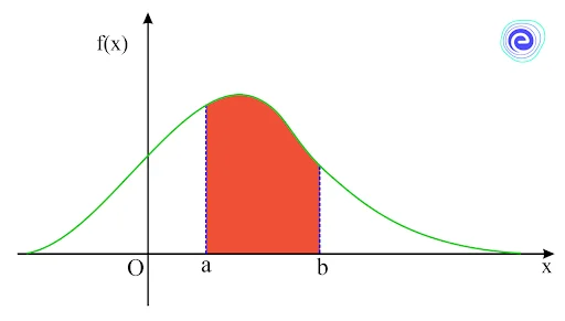
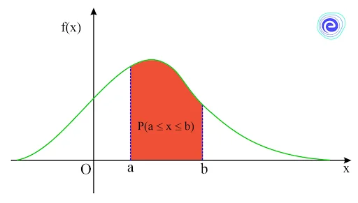
\({\text{P}}(a < {\text{X}} < {\text{b}}) = \int_a^b f (x)dx\)

Where, \(f(x)\) is the probability density function, \(a\) is the lower limit, and \(b\) is the upper limit.

Example

Let us consider a probability density function of some continuous random variable in \(f(x) = 2x – 1,\) when \(0 < x \le 2.\)

If we need to find the \({\rm{P}}(0.5 < {\rm{X}} < 1),\) we need to follow the steps given below:

• First, integrate the given function
  \(\int_{0.5}^1 (2 x – 1) = \left[ {{x^2}} \right]_{0.5}^1\)
• Now, apply the limits \(0.5\) and \(1\) and subtract the values obtained
  \({(1)^2} – {(0.5)^2} = 1 – 0.25 = 0.75\)

Thus, the result obtained gives the probability that the continuous random variable is within the given limits.

Here, the probability of the given continuous random variable lying between \(0.5\) and \(1\) is \(0.75.\)

Properties of a Probability Density Function

The properties of the probability density function assist in the faster resolution of problems. The following properties are relevant if \(f(x)\) is the probability distribution of a continuous random variable, \(X:\)

• The probability density function \(f(x)\) is never negative or cannot be less than zero.
• Thus, the probability density function is always greater than or equal to zero for all real numbers.
  \(f(x) \ge 0\)
• The total area under the probability density curve is always equal to one.
  \(\int_{ – \infty }^\infty f (x)dx = 1\)
• The probability density function curve is continuous over the entire range due to the property of continuous random variables. This also defines itself over a range of continuous values, or the variable’s domain.

LEARN EXAM CONCEPTS ON EMBIBE

Probability Density Function of Continuous Random Variable

A probability density function is the first derivative of the cumulative distribution function of a continuous random variable. A cumulative distribution function is obtained by integrating the probability density function.

Let \(X\) be the continuous random variable and \(F(x)\) be the cumulative distributive function of \(X.\) Then, the probability density function \(f(x)\) is given by

\(f(x) = \frac{{{\rm{dF}}(x)}}{{{\rm{dx}}}} = {{\rm{F}}^{\rm{I}}}(x) = F(x)\)

The probability of the random variable \(X,\) can be found by 

\({\rm{P}}(a < x \le b) = \int_a^b f (x)dx = F(b) – F(a)\)

Here, 

• \(a\) and \(b?\) lower and upper limits of the function 
• \(F(b)\) and \(F(a)?\) cumulative distribution functions at the values of \(a\) and \(b\)

Mean of Probability Density Function

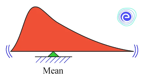
The expected (average) value of a random variable is the mean of a probability density function. The mean is obtained by the following formula if \(f(x)\) is the probability density function of the random variable

\(\mu = \int_{ – \infty }^\infty x \cdot f(x)dx\)

Median of Probability Density Function

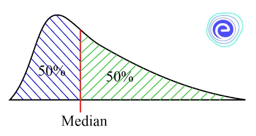
The median is the point on the probability density function curve that divides the curve into two equal halves. Assume that \(x=m\) is the median value. The area under the curve from \(-∞\) to \(m\) will be equal to the area from \(m\) to \(∞.\) This indicates that the median value is \(\frac{1}{2}.\) Hence, the probability density function’s median is as follows.

\({\mathop{\rm Median}\nolimits} = \int_{ – \infty }^m f (x)dx =\)

\(\int_m^\infty f (x)dx = \frac{1}{2}\)

Variance of Probability Density Function

The variance of a random variable is the expected value of the squared deviation from the mean. We can express this concept numerically as,

\({\mathop{\rm Var}\nolimits} (X) = E{(X – \mu )^2}\)

The variance of \(X,\) a random variable, is represented by the probability density function as follows.

\({\sigma ^2} = \int_{ – \infty }^\infty {{{({\rm{X}} – \mu )}^2}} f(x)dx\)

Applications of Probability density Function

The probability density function is helpful in various domains, including Statistics, Science, and Engineering. It has several interesting applications, which are listed below.

• It is used to calculate the probability associated with random variables in Statistics.
• The probability density function is used to represent the annual data of atmospheric \(N{O_x}\) temporal concentrations.
• It is used to simulate the combustion of a diesel engine.

Key Points

The below points give essential information about the probability density function.

• The probability density function calculates the likelihood that a continuous random variable will fall inside a given range of values.
• The value of the probability density function is always greater than one.
• The probability density function is the differentiation of the cumulative distribution function.
• The probability density function’s mean can be written as
  \({\rm{E}}(x) = \mu = \int_{ – \infty }^\infty x \cdot f(x)dx\)
• The median divides the probability density function curve into two halves; hence its value is \(\frac{1}{2}.\)
• Var is the variance of a probability density function is
  \({\mathop{\rm Var}\nolimits} ({\rm{X}}) = {\sigma ^2} = \int_{ – \infty }^\infty {{{({\rm{X}} – \mu )}^2}} f(x)dx\)

Solved Examples – Probability Density Function

Q1. Find the mean or exact value of \(X,\) for the probability density function is 

\(f(x) = \left\{ {\begin{array}{*{20}{l}} {\frac{{3{x^2}}}{2},}&{0 \le x \le 2}\\ {0,}&{{\rm{ otherwise }}} \end{array}} \right.\)

Solution:

We know that mean or expected value of the probability density function is given by

\({\rm{E}}(x) = \int_{ – \infty }^\infty x \cdot f(x)dx\)

So, mean of the given function is given by

\(\mu = \int_{ – \infty }^0 x \cdot (0)dx + \int_0^2 x \cdot \left( {\frac{{3{x^2}}}{2}} \right)dx + \int_2^\infty x \cdot (0)dx\)

\(\mu = \frac{3}{2}\left[ {\frac{{{x^4}}}{4}} \right]_0^2\)

\(\mu = \frac{3}{8}\left[ {{2^4} – {0^4}} \right]\)

\(\mu = \frac{3}{8} \times 16\)

\(\mu = 6\)

Hence, the mean of the given function is \(6.\)

Q2. The probability density function for the continuous variable \(X\) is given by 

\(f(x) = \left\{ {\begin{array}{*{20}{l}} {\frac{{b{e^{ – x}}}}{2},\quad x \ge 0}\\ {0,{\rm{ otherwise }}} \end{array}} \right.\), find the value of \(b.\)

Solution:

We know that, by the properties of probability density function the area under the curve of probability density function with the given limits is one.

Thus,  \(\int_{ – \infty }^\infty f (x)dx = 1\)

\(\int_0^\infty {\frac{{b{e^{ – x}}}}{2}} dx = 1\)

\(\frac{b}{2}\left[ { – {e^{ – x}}} \right]_0^\infty = 1\)

\(\frac{b}{2} = 1\)

\(∴b=2\)

Q3. Find \(P(1 < X \le 2).\) The given probability density function \(f(x) = \left\{ {\begin{array}{*{20}{l}} {(x – 1),0 \le x < 3}\\ {x,x \ge 3} \end{array}} \right.\) for a continuous random variable \(X.\)

Solution:

We know that the probability of the probability density function can be calculated by integrating the function within the given limits.

Thus, \({\rm{P}}(a < {\rm{X}} < {\rm{b}}) = \int_a^b f (x)dx\)

So, \({\rm{P}}(1 < {\rm{X}} \le 2) = \int_1^2 x (x – 1)dx\)

\( = \int_1^2 {\left( {{x^2} – x} \right)} dx\)

\( = \left[ {\frac{{{x^3}}}{3} – \frac{{{x^2}}}{2}} \right]_1^2\)

\( = \left[ {\frac{{{2^3}}}{3} – \frac{{{1^3}}}{3}} \right] – \left[ {\frac{{{2^2}}}{2} – \frac{{{1^2}}}{2}} \right] = \frac{5}{6}\)

\(\therefore {\rm{P}}(1 < X \le 2) = \frac{5}{6}\)

Q4. For the probability density function \(f(x) = x + 2,\) when \(0 < x \le 2,\) find \(P(0.5 < X < 1)\) of the continuous random variable \(X.\)

Solution:

Given: Probability density function of some continuous random variable is \(f(x) = 2x – 1,\) when \(0 < x \le 2.\) 

We know that the probability of a probability density function can be calculated by integrating the function within the given limits.

Thus, \({\rm{P}}(a < {\rm{X}} < {\rm{b}}) = \int_a^b f (x)dx\)

\({\rm{P}}(0.5 < {\rm{X}} < 1) = \int_{0.5}^1 {(x + 2)} dx\)  

\({\rm{P}}(0.5 < {\rm{X}} < 1) = \left[ {\frac{{{x^2}}}{2}} \right]_{0.5}^1\)

\({\rm{P}}(0.5 < {\rm{X}} < 1) = \left[ {\frac{{{1^2}}}{2} – \frac{{{{(0.5)}^2}}}{2}} \right]\)

\({\rm{P}}(0.5 < {\rm{X}} < 1) = 1.375\)

Here, the probability of the given continuous random variable lying between \(0.5\) and \(1\) is \(1.375.\)

Q5. Find the mean value of \(X,\) for the probability density function given is 

\(f(x) = \left\{ {\begin{array}{*{20}{l}} {2x – 1,\quad 0 \le x \le 3}\\ {0,{\rm{ otherwise }}} \end{array}} \right.\)

Solution:

We know that mean or expected value of the probability density function is given by

 \({\rm{E}}(x) = \int_{ – \infty }^\infty x \cdot f(x)dx\)

So, mean of the given function is given by

\(\mu = \int_{ – \infty }^0 x \cdot (0)dx + \int_0^2 x \cdot (2x – 1)dx + \int_2^\infty x \cdot (0)dx\) 

\(\mu = \int_0^2 {\left( {3{x^2} – 2x} \right)} dx\) 

\(\mu = 3\left[ {\frac{{{x^3}}}{3}} \right]_0^2 – 2\left[ {\frac{{{x^2}}}{2}} \right]_0^2\) 

 \(\mu = \left[ {{x^3}} \right]_0^2 – \left[ {{x^2}} \right]_0^2\)

\(\mu = \left( {{2^3} – {0^3}} \right) – \left( {{2^2} – {0^2}} \right)\) 

\(\mu = 8 – 4\)

\(\therefore \mu = 4\)

Summary

A probability density function (PDF) is used in probability theory to characterise the random variable’s likelihood of falling into a specific range of values rather than taking on a single value. The function illustrates the normal distribution’s probability density function and how mean and deviation are calculated. The standard normal distribution is used to generate databases and statistics, and it is frequently used in Science to represent real-valued variables with unknown distributions. The probability curve’s area under the curve is one. The probability density function’s median \(\frac{1}{2}.\) The mean of the random variable is the integration of the curve, and it is also known as the expected value.

Frequently Asked Questions (FAQs)

The frequently asked questions on probability density function are given below:

Q.1. What is meant probability density function?
Ans: The probability density function is a function that calculates the likelihood of a continuous random variable falling within a given interval. This probability is calculated using the integral of the probability density function.

Q.2. Does the probability function have a negative value?
Ans: A probability density function’s integral will always have a positive value. This is because probability can never be negative.

Q.3. What is the formula of probability density function?
Ans: The probability density function is obtained by differentiating the cumulative distribution function of a continuous random variable.
\(F(x)\) be the cumulative distributive function of \(X.\) Then, the probability density function \(f(x)\) is given by
\(f(x) = \frac{{{\rm{dF}}({\rm{x}})}}{{{\rm{dx}}}} = {{\rm{F}}^{\rm{I}}}({\rm{x}})\)

Q.4. How to find the mean of the probability density function?
Ans: The expected value or mean value of the probability density function can be calculated by using the formula
\(\mu = \int_{ – \infty }^\infty x .f(x)dx\)

Q.5. How do you calculate the probability of a probability density function?
Ans: The probability of a probability density function \(f(x)\) with the limits \(a\) and \(b\) is given by
\({\rm{P}}(a < {\rm{X}} < {\rm{b}}) = \int_a^b f (x)dx\)

Q.6. How do you find the probability density function of a discrete variable?
Ans: We use the probability mass function similar to the probability density function for discrete random variables. The value of a probability density function is calculated for a set of values for continuous variables, and at a particular point for discrete variables.

ATTEMPT MATHS MOCK TESTS

We hope this detailed article on the Probability of Density Function has helped you. If you have any doubts or queries, please leave a comment down below. We will be more than happy to help you.