Random variables and its probability distributions: A variable that is used to quantify the outcome of a random experiment is a random variable. Since there are two forms of data, discrete and continuous, there are two types of random variables. A discrete random variable can have an exact value, whereas the value of a continuous random variable will lie within a specific range.

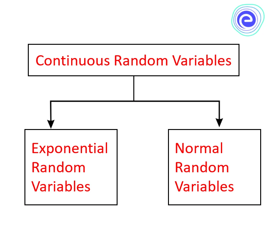
Exponential and normal random variables are the types of continuous random variables, while binomial, Poison’s, Bernoulli’s, and geometric are the types of discrete random variables. Probability distribution is a function that calculates the likelihood of all possible values for a random variable.

Definition of Random Variable

A random variable is a type of variable whose value is determined by the numerical results of a random experiment. A random variable is also called a stochastic variable. As random variables must be quantifiable, they are always real numbers.

Random Variable vs Algebraic Variable

A random variable can have different values because a random event might have multiple outcomes. As a result, do not even confuse a random variable with an algebraic variable. In an algebraic equation, an algebraic variable represents the value of an unknown quantity. On the other hand, a random variable can have a collection of values that could be the result of a random experiment.

Example: Assume two dice are rolled, and the random variable \(X\) represents the sum of the numbers. The smallest value of \(X\) will be \(2\) , while the largest possible value is \(12\) . As a result, \(X\) may be any number equal to or between \(2\) and \(12\) . After assigning probabilities to each outcome, the probability distribution of \(X\) may be calculated.

Properties of Random Variable

• Random variables take only positive real values
• If \(C\) is any real number and \(X\) is any random variable, then \(CX\) is a random variable.
• If \(x\) and \(y\) are two random variables, then
  (i) \(x+y\) is a random variable
  (ii) \(xy\) is a random variable

• For any constants \(\mathrm{K}\) and \(\mathrm{C}, \mathrm{K} x+\mathrm{C} y\) is also a random variable.
• The modulus \((|X|)\) is also a random variable for any random variable \(\mathrm{X}\).

Types of Random Variables

Random variables can be categorised based on the available data type, as shown below.

Continuous Random Variable

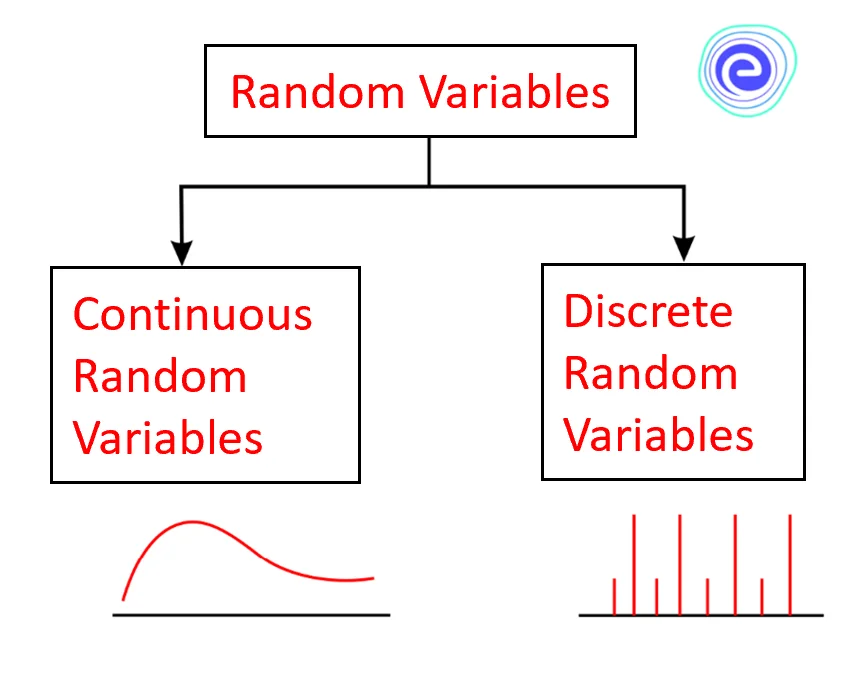
A continuous random variable is that which has infinite possible values. A variable like this is defined over a range of values rather than a single value. The weight of a person is an example of a continuous random variable. A probability density function is used to describe a continuous random variable because the probability that it will take on an exact value is zero.

Types of Continuous Random Variables

Exponential Continuous Random Variable

Exponential random variable	\(\mathrm{X} \sim \operatorname{Exp}(\lambda)\)
The probability density function of the exponential random variable	\(f(x) = \left\{ {\begin{array}{*{20}{c}}{\lambda {e^{ – \lambda x}},}&{x \ge 0}\\{0,}&{x < 0}\end{array}} \right\}\)

Normal Continuous Random Variable

Normal random variable	\(\mathrm{X} \sim\left(\mu, \sigma^{2}\right)\)
Probability density function	\(f(x)=\frac{1}{\sigma \sqrt{2 \pi}} e^{-\frac{1}{2}\left(\frac{x-\mu}{\sigma}\right)^{2}}\)

Discrete Random Variable

A discrete random variable can have a finite number of different values. For example, a discrete random variable can be used to represent the number of children in a family. A probability distribution is used to determine what values a random variable can take and how frequently it does so. 

Types of Discrete Random Variables

Binomial Discrete Random Variable

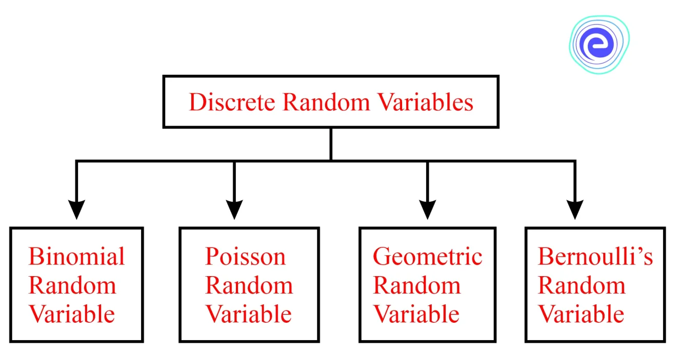
A binomial random variable indicates the number of successes in a binomial experiment. A binomial experiment consists of a set number of repeated Bernoulli trials with only two possible outcomes: success or failure. The number of trials is denoted by \(n\), while the chance of success is denoted by \(p\).

Binomial random variable	\(\mathrm{X} \sim \operatorname{Bin}(n, p)\)
Probability density function	\(P\left( {X = x} \right) = \left( {\begin{array}{*{20}{c}} n \\ x \end{array}} \right){p^x}{\left( {1 – p} \right)^{n – x}}\)

Geometric Discrete Random Variable

In a Bernoulli trial, the probability of success is \(p\), and the probability of failure is \(1-p\).

Geometric random variable	\(\mathrm{X} \sim \mathrm{G}(\mathrm{p})\)
Probability density function	\(P(X=x)=(1-p)^{x-1} p\)

Bernoulli’s Discrete Random Variable

The simplest sort of random variable is Bernoulli’s random variable. There are only two possible values for this variable: \(1\) for success and \(0\) for failure.

Bernoulli’s random variable	\(X \sim\) Bernoulli \((p)\)
Probability density function	\(P(X = x) = \left\{ {\begin{array}{*{20}{c}}{p,}&{{\text{if}}\,\,x = 1}\\{1 – p,}&{{\text{if}}\,\,x = 0}\end{array}} \right\}\)

Poisson Discrete Random Variable

A Poisson random variable illustrates how many times an event will happen in the given time. These events occur at a consistent rate and in random order.

Poisson discrete random variable	\(X \sim\) Poisson \((\lambda)\)
Probability density function	\(P(X=x)=\frac{\lambda^{x} e^{-\lambda}}{x !}\)

Mean of a Random Variable

The weighted average of all the values of a random variable can also be described as the mean or expected value of the variable. It is represented by \(E[X]\). Here, \(X\) is the random variable. The following are the formulas for calculating the mean of a random variable:

Mean of discrete random variable	\(E\left[ X \right] = \sum {xP\left( {X = x} \right)}\) where \({P\left( {X = x} \right)}\) is the probability mass function.
Mean of continuous random variable	\(E\left[ X \right] = \int {xf\left( x \right)dx}\) where \(f\left( x \right)\)  is the probability density function

Variance of a Random Variable

Variance of a random variable is the expected value of the square of the difference between the random variable and the mean. Var\([X]\) or \(\sigma^{2}\) represents the variance of a random variable. If \(\mu\) is the mean, then the variance can be calculated as follows:

Variance of continuous random variable	\(\operatorname{Var}[\mathrm{X}]=\int(\mathrm{x}-\mu)^{2} \mathrm{f}(\mathrm{x}) \mathrm{dx}\)
Variance of discrete random variable	\(\operatorname{Var}[\mathrm{X}]=\sum(\mathrm{x}-\mu)^{2} \mathrm{P}(\mathrm{X}=\mathrm{x})\)

Definition of Probability Distribution

A probability distribution is a function that calculates the likelihood of all possible values for a random variable. A probability distribution and probability mass functions can both be used to define a discrete probability distribution. A continuous probability distribution is described using a probability distribution function and a probability density function.

Probability Distribution Function

The probability distribution function is also known as the cumulative distribution function (CDF). This gives the likelihood of a random variable, \(\mathrm{X}\). When evaluated at a point, \(x\), it takes values less than or equal to \(x\).

\(F(x)=P(X \leq x)\)

Furthermore, if \((a, b]\) is a semi-closed interval, the probability distribution function is provided by the formula given below.

\(\mathrm{P}(\mathrm{a}<\mathrm{X} \leq \mathrm{b})=\mathrm{F}(\mathrm{b})-\mathrm{F}(\mathrm{a})\)

A random variables probability distribution function is always between \(0\) and \(1\) . It is a function that does not decrease.

Formulas of Probability Distribution

A probability distribution has multiple formulas depending on the type of distribution a random variable follows.

Probability Distribution of a Discrete Random Variable

For a discrete random variable, the formulas for the probability distribution function and the probability mass function are as follows:

Probability distribution function	\(\mathrm{F}(\mathrm{x})=\mathrm{P}(\mathrm{X} \leq \mathrm{x})\)
Probability mass function	\(\mathrm{p}(\mathrm{x})=\mathrm{P}(\mathrm{X}=\mathrm{x})\)

Probability Distribution of a Continuous Random Variables

We cannot use the probability mass function to characterise such distribution since the likelihood that a continuous random variable would take on an exact value is \(0\) . Hence, we use the probability density function.

Probability distribution function	\(F(x)=P(X \leq x)\)
Probability mass function	\(\mathrm{f}(\mathrm{x})=\frac{\mathrm{d}}{\mathrm{dx}}(\mathrm{F}(\mathrm{x}))\), where \({\rm{F}}({\rm{x}}) = \int_{ – \infty }^x f (u)du\)

Solved Examples of Random Variables and its Probability Distributions

Here are a few solved examples for the students,

Q.1. If two dice are rolled, what is the probability distribution of the sum of the dice?
Sol: 
Possible outcomes \(=(2,3,4,5,6,7,8,9,10,11,12)\)
Assume \(1\) is rolled on the first die and \(1\) is rolled on the second die.
The total will then be \(2\) , because no alternative set of integers can produce the same result.
Probability of having the result is \(2=\frac{1}{36}\).
Other numbers are treated in the same way.

\(x\)	\(2\)	\(3\)	\(4\)	\(5\)	\(6\)	\(7\)	\(8\)	\(9\)	\(10\)	\(11\)	\(12\)
\(P(x)\)	\(\frac{1}{36}\)	\(\frac{2}{36}\)	\(\frac{3}{36}\)	\(\frac{4}{36}\)	\(\frac{5}{36}\)	\(\frac{6}{36}\)	\(\frac{5}{36}\)	\(\frac{4}{36}\)	\(\frac{3}{36}\)	\(\frac{2}{36}\)	\(\frac{1}{36}\)

Q.2. Find the probability that a die will show a number less than \(6\), if rolled multiple times.
Sol:
Possible outcomes are \(\left\{ {1,2,3,4,5,6} \right\}\)
Numbers less than \(6 = \left\{ {1,2,3,4,5} \right\}\)
\(\mathrm{P}(\mathrm{X}<6)=\mathrm{P}(\mathrm{X}=1)+\mathrm{P}(\mathrm{X}=2)+\mathrm{P}(\mathrm{X}=3)+\mathrm{P}(\mathrm{X}=4)+\mathrm{P}(\mathrm{X}=5)\)
\(P(X<6)=\frac{1}{6}+\frac{1}{6}+\frac{1}{6}+\frac{1}{6}+\frac{1}{6}=\frac{5}{6}\)
\(\therefore \mathrm{P}(\mathrm{X}<6)=\frac{5}{6}\)

Q.3. The probability mass function is given by \(p\left( x \right) = \left\{ {\begin{array}{*{20}{c}} \begin{gathered} 0.2, \hfill \\ 0.3, \hfill \\ 0.1, \hfill \\ 0.4, \hfill \\ 0, \hfill \\ \end{gathered} &\begin{gathered} x = 0.1 \hfill \\ x = 0.2 \hfill \\ x = 0.3 \hfill \\ x = 0.4 \hfill \\ {\text{otherwise}} \hfill \\ \end{gathered} \end{array}} \right.\) for a discrete variable \(x.\) Find the value of \(P(x<4)\)
Sol:
Given : \(p\left( x \right) = \left\{ {\begin{array}{*{20}{c}} \begin{gathered} 0.2, \hfill \\ 0.3, \hfill \\ 0.1, \hfill \\ 0.4, \hfill \\ 0, \hfill \\ \end{gathered} &\begin{gathered} x = 0.1 \hfill \\ x = 0.2 \hfill \\ x = 0.3 \hfill \\ x = 0.4 \hfill \\ {\text{otherwise}} \hfill \\ \end{gathered} \end{array}} \right.\)
The value of \(P(x<4)=P(X=1)+P(X=2)+P(X=3)\)
\(P(x<4)=0.2+0.3+0.1\)
\(\therefore P(x<4)=0.6\)

Q.4. Assume that you have a \(25 \%\) chance of hitting the bullseye in a game of darts. What are the chances of hitting the bullseye five times if you take a total of \(15\) shots?
Sol:
Given \(n=15, x=5\) and \(P=25 \%=\frac{25}{100}=\frac{1}{4}\)
The binomial probability distribution function is given by
\(P\left( {X = x} \right) = \left( {\begin{array}{*{20}{c}} n \\ x \end{array}} \right){p^x}{\left( {1 – p} \right)^{n – x}}\)
\(P\left( {X = 5} \right) = \left( {\begin{array}{*{20}{c}} {15} \\ 5 \end{array}} \right){0.25^5}{\left( {1 – 0.25} \right)^{15 – 5}}\)
\( = \left( {\begin{array}{*{20}{c}} {15} \\ 5 \end{array}} \right){0.25^5}{\left( {0.75} \right)^{10}}\)
\(\therefore P(X=5)=0.165\)

Q.5. Find the mean of the following distribution function \(F\left( x \right) = \left\{ {\begin{array}{*{20}{c}} {\left( {p + 1} \right){x^{p + 1}},}&{0 \leqslant x \leqslant 1} \\ {0,}&{{\text{otherwise}}} \end{array}} \right.\)
Sol:
Given: \(p>-1\)
The mean of the distribution is given by \(\mathrm{E}(\mathrm{x})=\int x . f(x) d x\)
So, \(E(x)=\int_{0}^{1}(p+1) x^{p+1} d x\)
\(E(x)=\left[\frac{(p+1) x^{p+2}}{p+2}\right]_{0}^{1}\)
\(\therefore E(x)=\frac{p+1}{p+2}\)

Summary

A random variable is used to quantify a random experiment’s outcome. There are two forms of data, discrete and continuous. Hence, there are two types of random variables. A discrete random variable can have an exact value, whereas the value of a continuous random variable will lie within a specific range.

Exponential and normal are the types of continuous random variables. Geometric, binomial, and Bernoulli are the types of discrete random variables. A probability distribution is a function that calculates the likelihood of all possible values for a random variable. Probability distributions are diagrams that depict how probabilities are spread throughout the values of a random variable.

FAQs of Random Variables and its Probability Distributions

Students must have many questions with respect to Random Variables and its Probability Distributions. Here are a few commonly asked questions and answers.

Q.1. What is meant by random variable?
Ans: A random variable is that which represents all possible outcomes of a random event.

Q.2. What are two types of random variables?
Ans: Random variables are of two types: discrete random variables and continuous random variables. A discrete random variable can have a single value, while a continuous random variable has a range of values.

Q.3. What is a probability distribution?
Ans: The probability that a random variable will take on a specific value is represented by a probability distribution.

Q.4. What are the types of probability distributions?
Ans: The various types of probability distributions include binomial, Bernoulli’s, normal, and geometric distributions.

Q.5. What is the difference between discrete and continuous random variables?
Ans: A discrete random variable can have an exact value, whereas a continuous random variable’s value will lie within a specific range.

We hope this information about Random Variables and its Probability Distributions has been helpful. If you have any doubts, comment in the section below, and we will get back to you soon.